Hi!
Very good blog...
I'm doing some stuff with Clementine... and I have an issue...
My target for NN train dataset is a continuos value between 0 and 100... the problem is that is a normal/gaussian distribution and makes the NN predict bad...
How can I resolve the unbalancing data? split into classe with same frequency!?
Regards,
Pedro
Pedro,
I am not aware that neural networks have a problem with predicting values with normal distributions. In fact, if you randomize the weights in a neural network whose output layer has a linear transfer function, then the output is likely to follow a normal distribution -- just from the Central Limit Theorem of statistics.
So, you have a neural network that is not producing good results. There can be several causes.
The first thing to look for is too many inputs. Clementine has options to prune the input variables on a neural network. Be sure that you do not have too many inputs. I would recommend a variable reduction technique such as principal components, and advise you to avoid categorical variables that have many levels.
A similar problem can occur if your hidden layer is too large.
Whatever the network, it is worthwhile looking at the number of weights in the network (or a related measure called the degrees of freedom). Remember, you want to have lots of training data for each weight.
Another problem may be that the target is continuous, but bounded between 0 and 100. This could result in a neural network where the output layer uses a linear transfer function. Although not generally a bad idea, it may not work in this case because the range of a linear function is from minus infinity to positive infinity, which far exceeds the range of the data.
One simple solution would be to divide the output by 100 and treat it as a probability. The neural network should then be set up with a logistic function in the target layer.
Your idea of binning the results might also work, assuming that bins work for solving the business problem. Equal sized bins are reasonable, since they are readily understandable as quantiles.
Good luck.
Showing posts with label Neural Networks. Show all posts
Showing posts with label Neural Networks. Show all posts
Tuesday, August 25, 2009
Sunday, January 18, 2009
Thoughts on Understanding Neural Networks
Lately, I've been thinking quite a bit about neural networks. In particular, I've been wondering whether it is actually possible to understand them. As a note, this posting assumes that the reader has some understanding of neural networks. Of course, we at Data Miners, heartily recommend our book Data Mining Techniques for Marketing, Sales, and Customer Relationship Management for introducing neural networks (as well as a plethora of other data mining algorithms).
Let me start with a picture of a neural network. The following is a simple network that takes three inputs and has two nodes in the hidden layer:
 Note that this structure of the network explains what is really happening. The "input layer" (the first layer connected to the inputs) standardizes the inputs. The "output layer" (connect to the output) is doing a regression or logistic regression, depending on whether the target is numeric or binary. The hidden layers are actually doing a mathematical operation as well. This could be the logistic function; more typically, though it is the hyperbolic tangent. All of the lines in the diagram have weights on them. Setting these weights -- plus a few others not shown -- is the process of training the neural network.
The topology of the neural network is specifically how SAS Enterprise Miner implements the network. Other tools have similar capabilities. Here, I am using SAS EM for three reasons. First, because we teach a class using this tool, I have pre-built neural network diagrams. Second, the neural network node allows me to score the hidden units. And third, the graphics provide a data-colored scatter plot, which I use to describe what's happening.
There are several ways to understand this neural network. The most basic way is "it's a black box and we don't need to understand it." In many respects, this is the standard data mining viewpoint. Neural networks often work well. However, if you want a technique that let's you undersand what it is doing, then choose another technique, such as regression or decision trees or nearest neighbor.
A related viewpoint is to write down the equation for what the network is doing. Then point out that this equation *is* the network. The problem is not that the network cannot explain what it is doing. The problem is that we human beings cannot understand what it is saying.
I am going to propose two other ways of looking at the network. One is geometrically. The inputs are projected onto the outputs of the hidden layer. The results of this projection are then combined to form the output. The other method is, for lack of a better term, "clustering". The hidden nodes actually identify patterns in the original data, and one hidden node usually dominates the output within a cluster.
Let me start with the geometric interpretation. For the network above, there are three dimensions of inputs and two hidden nodes. So, three dimensions are projected down to two dimensions.
I do need to emphasize that these projections are not the linear projections. This means that they are not described by simple matrices. These are non-linear projections. In particular, a given dimension could be stretched non-uniformly, which further complicates the situation.
I chose two nodes in the hidden layer on purpose, simply because two dimensions are pretty easy to visualize. Then I went and I tried it on a small neural network, using Enterprise Miner. The next couple of pictures are scatter plots made with EM. It has the nice feature that I can color the points based on data -- a feature sadly lacking from Excel.
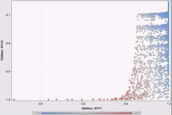
The following scatter plot shows the original data points (about 2,700 of them). The positions are determined by the outputs of the hidden layers. The colors show the output of the network itself (blue being close to 0 and red being close to 1). The network is predicting a value of 0 or 1 based on a balanced training set and three inputs.
 Hmm, the overall output is pretty much related to the H1 output rather than the H2 output. We see this becasuse the color changes primarily as we move horizontally across the scatter plot and not vertically. This is interesting. It means that H2 is contributing little to the network prediction. Under these particular circumstances, we can explain the output of the neural network by explaining what is happening at H1. And what is happening at H1 is a lot like a logistic regression, where we can determine the weights of different variables going in.
Note that this is an approximation, because H2 does make some contribution. But it is a close approximation, because for almost all input data points, H1 is the dominant node.
This pattern is a consequence of the distribution of the input data. Note that H2 is always negative and close to -1, whereas H1 varies from -1 to 1 (as we would expect, given the transfer function). This is because the inputs are always positive and in a particular range. The inputs do not result in the full range of values for each hidden node. This fact, in turn, provides a clue to what the neural network is doing. Also, this is close to a degenerate case because one hidden unit is almost always ignored. It does illustrate that looking at the outputs of the hidden layers are useful.
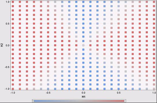
This suggests another approach. Imagine the space of H1 and H2 values, and further that any combination of them might exist (do remember that because of the transfer function, the values actually are limited to the range -1 to 1). Within this space, which node dominates the calculation of the output of the network?
To answer this question, I had to come up with some reasonable way to compare the following values:

There are four regions in this scatter plot, defined essentially by the intersection of two lines. In fact, each hidden node is going to add another line on this chart, generating more regions. Within each region, one node is going to dominate. The boundaries are fuzzy. Sometimes this makes no difference, because the output on either side is the same; sometimes it does make a difference.
Note that this scatter plot assumes that the inputs can generate all combinations of values from the hidden units. However, in practice, this is not true, as shown on the previous scatter plot, which essentially covers only the lowest eights of this one.
With the contribution metric, we can then say that for different regions in the hidden unit space, different hidden units dominate the output. This is essentially saying that in different areas, we only need one hidden unit to determine the outcome of the network. Within each region, then, we can identify the variables used by the hidden units and say that they are determining the outcome of the network.
This idea leads to a way to start to understand standard multilayer perceptron neural networks, at least in the space of the hidden units. We can identify the regions where particular hidden units dominate the output of the network. Within each region, we can identify which variables dominate the output of that hidden unit. Perhaps this explains what is happening in the network, because the input ranges limit the outputs only to one region.
More likely, we have to return to the original inputs to determine which hidden unit dominates for a given combination of inputs. I've only just started thinking about this idea, so perhaps I'll follow up in a later post.
--gordon
Let me start with a picture of a neural network. The following is a simple network that takes three inputs and has two nodes in the hidden layer:
 Note that this structure of the network explains what is really happening. The "input layer" (the first layer connected to the inputs) standardizes the inputs. The "output layer" (connect to the output) is doing a regression or logistic regression, depending on whether the target is numeric or binary. The hidden layers are actually doing a mathematical operation as well. This could be the logistic function; more typically, though it is the hyperbolic tangent. All of the lines in the diagram have weights on them. Setting these weights -- plus a few others not shown -- is the process of training the neural network.
The topology of the neural network is specifically how SAS Enterprise Miner implements the network. Other tools have similar capabilities. Here, I am using SAS EM for three reasons. First, because we teach a class using this tool, I have pre-built neural network diagrams. Second, the neural network node allows me to score the hidden units. And third, the graphics provide a data-colored scatter plot, which I use to describe what's happening.
There are several ways to understand this neural network. The most basic way is "it's a black box and we don't need to understand it." In many respects, this is the standard data mining viewpoint. Neural networks often work well. However, if you want a technique that let's you undersand what it is doing, then choose another technique, such as regression or decision trees or nearest neighbor.
A related viewpoint is to write down the equation for what the network is doing. Then point out that this equation *is* the network. The problem is not that the network cannot explain what it is doing. The problem is that we human beings cannot understand what it is saying.
I am going to propose two other ways of looking at the network. One is geometrically. The inputs are projected onto the outputs of the hidden layer. The results of this projection are then combined to form the output. The other method is, for lack of a better term, "clustering". The hidden nodes actually identify patterns in the original data, and one hidden node usually dominates the output within a cluster.
Let me start with the geometric interpretation. For the network above, there are three dimensions of inputs and two hidden nodes. So, three dimensions are projected down to two dimensions.
I do need to emphasize that these projections are not the linear projections. This means that they are not described by simple matrices. These are non-linear projections. In particular, a given dimension could be stretched non-uniformly, which further complicates the situation.
I chose two nodes in the hidden layer on purpose, simply because two dimensions are pretty easy to visualize. Then I went and I tried it on a small neural network, using Enterprise Miner. The next couple of pictures are scatter plots made with EM. It has the nice feature that I can color the points based on data -- a feature sadly lacking from Excel.
The following scatter plot shows the original data points (about 2,700 of them). The positions are determined by the outputs of the hidden layers. The colors show the output of the network itself (blue being close to 0 and red being close to 1). The network is predicting a value of 0 or 1 based on a balanced training set and three inputs.
 Hmm, the overall output is pretty much related to the H1 output rather than the H2 output. We see this becasuse the color changes primarily as we move horizontally across the scatter plot and not vertically. This is interesting. It means that H2 is contributing little to the network prediction. Under these particular circumstances, we can explain the output of the neural network by explaining what is happening at H1. And what is happening at H1 is a lot like a logistic regression, where we can determine the weights of different variables going in.
Note that this is an approximation, because H2 does make some contribution. But it is a close approximation, because for almost all input data points, H1 is the dominant node.
This pattern is a consequence of the distribution of the input data. Note that H2 is always negative and close to -1, whereas H1 varies from -1 to 1 (as we would expect, given the transfer function). This is because the inputs are always positive and in a particular range. The inputs do not result in the full range of values for each hidden node. This fact, in turn, provides a clue to what the neural network is doing. Also, this is close to a degenerate case because one hidden unit is almost always ignored. It does illustrate that looking at the outputs of the hidden layers are useful.
This suggests another approach. Imagine the space of H1 and H2 values, and further that any combination of them might exist (do remember that because of the transfer function, the values actually are limited to the range -1 to 1). Within this space, which node dominates the calculation of the output of the network?
To answer this question, I had to come up with some reasonable way to compare the following values:
- Network output: exp(bias + a1*H1 + a2*H2)
- H1 only: exp(bias + a1*H1)
- H2 only: exp(bias + a2*H2)
- Network output: 0.9994
- H1 only output: 0.9926
- H2 only output: 0.9749
- H1 contribution: (0.9994 - 0.9926)^2 / ((0.9994 - 0.9926)^2 + (0.9994 - 0.9749)^2)
There are four regions in this scatter plot, defined essentially by the intersection of two lines. In fact, each hidden node is going to add another line on this chart, generating more regions. Within each region, one node is going to dominate. The boundaries are fuzzy. Sometimes this makes no difference, because the output on either side is the same; sometimes it does make a difference.
Note that this scatter plot assumes that the inputs can generate all combinations of values from the hidden units. However, in practice, this is not true, as shown on the previous scatter plot, which essentially covers only the lowest eights of this one.
With the contribution metric, we can then say that for different regions in the hidden unit space, different hidden units dominate the output. This is essentially saying that in different areas, we only need one hidden unit to determine the outcome of the network. Within each region, then, we can identify the variables used by the hidden units and say that they are determining the outcome of the network.
This idea leads to a way to start to understand standard multilayer perceptron neural networks, at least in the space of the hidden units. We can identify the regions where particular hidden units dominate the output of the network. Within each region, we can identify which variables dominate the output of that hidden unit. Perhaps this explains what is happening in the network, because the input ranges limit the outputs only to one region.
More likely, we have to return to the original inputs to determine which hidden unit dominates for a given combination of inputs. I've only just started thinking about this idea, so perhaps I'll follow up in a later post.
--gordon
Wednesday, January 14, 2009
Neural Network Training Methods
Scott asks . . .
Dear Ask a Data Miner,
I am using SPSS Clementine 12. The Neural Network node in Clementine allows users to choose from six different training methods for building neural network models:
• Quick. This method uses rules of thumb and characteristics of the data to choose an appropriate shape (topology) for the network.
• Dynamic. This method creates an initial topology but modifies the topology by adding and/or removing hidden units as training progresses.
• Multiple. This method creates several networks of different topologies (the exact number depends on the training data). These networks are then trained in a pseudo-parallel fashion. At the end of training, the model with the lowest RMS error is presented as the final model.
• Prune. This method starts with a large network and removes (prunes) the weakest units in the hidden and input layers as training proceeds. This method is usually slow, but it often yields better results than other methods.
• RBFN. The radial basis function network (RBFN) uses a technique similar to k-means clustering to partition the data based on values of the target field.
• Exhaustive prune. This method is related to the Prune method. It starts with a large network and prunes the weakest units in the hidden and input layers as training proceeds. With Exhaustive Prune, network training parameters are chosen to ensure a very thorough search of the space of possible models to find the best one. This method is usually the slowest, but it often yields the best results. Note that this method can take a long time to train, especially with large datasets.
Which is your preferred training method? How about for a lot of data - (a high number of cases AND a high number of input variables)? How about for a relatively small amount of data?
Scott,
Our general attitude with respect to fancy algorithms is that they provide incremental value. However, focusing on data usually provides more scope for improving results. This is particularly true of neural networks, because stable neural networks should have few inputs.
Before addressing your question, there are a few things that you should keep in mind when using neural networks:
(1) Standardize all the inputs (that is, subtract the average and divide by the standard deviation). This puts all numeric inputs into a particular range.
(2) Avoid categorical inputs! These should be replaced by appropriate numeric descriptors. Neural network tools, such as Clementine, handle categorical inputs using something called n-1 coding, which converts one variable into many flag variables, which, in turn, multiplies the number of weights in the network that need to be optimized.
(3) Avoid variables that are highly collinear. These cause "multidimensional ridges" in the space of neural network weights, which can confuse the training algorithms.
To return to your question in more detail. Try out lots of the different approaches to determine which is best! There is no rule that says that you have to decide on one approach initially and stick with it. To test the approaches use a separate partition of the data to see which works best.
For instance, the Quick method is probably very useful in getting results back in a reasonable amount of time. Examine the topology, though, to see if it makes sense (no hidden units or too many hidden units). Most of the others are all about adding or removing units, which can be valuable. However, always test the methods on a test set that is not used for training. The topology of the network may depend on the training set, so that provides an opportunity for overfitting.
These methods are focusing more on the topology than on the input parameters. If the prune method really does remove inputs, then that would be powerful functionality. For the methods that are comparing results, ensure that the results are compared on a validation set, separate from the test set used to calculate the weights. It can be easy to overfit neural networks, particularly as the number of weights increases.
A comment about the radial basis function approach. Make sure that Clementine is using normalized radial basis functions. Standard neural networks use an s-shaped function that starts low and goes high (or vice versa), meaning that the area under the curve is unbounded. RBFs start low, go high, and then go low again, meaning that the area under the curve is finite. Normalizing the RBFs ensures that the basis functions do not get too small.
My personal favorite approach to neural networks these days is to use principal components as inputs into the network. To work effectively, this requires some background in principal components to choose the right number as inputs into the network.
--gordon
Subscribe to:
Posts (Atom)


