An Achievement on Stack Overflow

Last Friday (August 22nd), I achieved a milestone on Stack Overflow, a computing question-and-answer site, by hitting 200,000 points.  So far this year, I have also earned more points than anyone, a testament to my obsession with the site (you can see yearly user rankings here).  As for overall points, I will never match the leader Jon Skeet because who had a head start of many years.

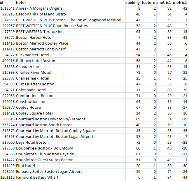
My answers are almost almost exclusively for answers related to SQL and various databases.   The site is highly geared toward "tools" questions, so there are few general analysis questions.

So, this blog is sharing some of my thoughts and my history on the site.

Clearly, I have helped a lot of people on Stack Overflow, around the world.  The most rewarding part are the thank-yous from real people working on real problems.  On several instances, I have helped speed up code by more than 99% -- turning hours of drudgery into seconds or minutes of response time.

But answering questions has helped me too:

• My technical knowledge of databases has greatly improved, particularly the peculiarities (strengths and weaknesses) of each database engine.
• I have learned patience for people who are confused by concepts in SQL.
• I have (hopefully) learned how to explain concepts to people with different levels of competence.
• I have learned how to figure out (sometimes) what someone is really asking.
• I have a strong appreciation for what SQL can do and what SQL cannot do.
• It has definitely increased the number of hits when I egosurf.

A few months after starting, I stopped down voting questions and answers.  "Down voting" is usually seen as "not-nice", making the other person defensive, confused, and perhaps angry.   A lesson for real life:  being mean (by down voting) is not nearly so useful as offering constructive criticism (by commenting).

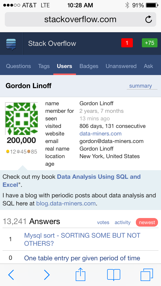
This all started in January, 2012 (a bit over two and a half years ago).  The reason was simple:  I was writing a system called The Netting Machine for the Lehman Brothers Estate and it was stretching my knowledge of SQL Server.  One particular problem involved dynamic queries.  Google kept directing me to the same question on Stack Overflow.  This best answer was close to what I needed, but not quite.  It was only half-way there.  The third time I landed on the page, I added my own answer.  This was actually for quite selfish reasons:  the next time Google took me there, I wanted to see the full answer.

Lo and behold, my answer was accepted and up voted.  When the OP ("original poster" -- Stack Overflow lingo for the person asking the question) accepted my answer, s/he had to unaccept another.  That answer was by Aaron Bertrand, a SQL Server guru whose name I recognized from his instructive blog posts.  Aaron commented about the "unaccept".  In the back of my mind, If Aaron thinks this is important, then there must be something to it.  Ultimately, I can blame Aaron (whom I have not yet met in person) for getting me hooked.

For a few months, I sporadically answered questions.  Then, in the first week of May, my Mom's younger brother passed away.  That meant lots of time hanging around family, planning the funeral, and the like.  Answering questions on Stack Overflow turned out to be a good way to get away from things.  So, I became more intent.

Stack Overflow draws you in not only with points but with badges and privileges.  Each time I logged in, the system "thanked" me for my participation with more points, more badges, and more privileges.   This continued.  One day (probably in June), I hit the daily upvote maximum of 200 upvotes (you also get points when an answer is accepted or someone offers a bounty).  One week, I hit 1000 points.  One month, 5,000 points.  As an individual who is mesmerized by numbers, I noticed these things.

Last summer, I hit 100,000 points in September and slowed down.  I figured that six figures was enough, and I had other, more interesting things to do -- a trip to Myanmar, my sister's wedding, our apartment in Miami, classes to teach (San Francisco, Amsterdam, Chicago, San Antonio, Orlando) and so on.

I didn't start 2014 with the intention of spending too much of my time on the site.  But three things happened in January.  The first was a fever with a rash on my face.  It kept me home with not-enough to do.  So, I answered questions on Stack Overflow.  Then, I had an attack of gout.  That kept me home with not-enough to do.  And finally, the weather in January in New York was, well, wintery -- lots of cold and lots of snowy.  More reasons to stay home and answer questions.

By the end of January, I was the top scorer for the month.  "Hey, if I can do it in January, let's see what happens in February."  I had thought of relenting in April:   we flew to Greece and spent two nights on Mount Athos.  Mount Athos is a peninsula in northern Greece, devoted to twenty-one Orthodox monasteries -- and nothing else.  It is inhabited by a few thousand monks living medieval lifestyles.  The only way to visit is as a "pilgrim", staying at a monastery.  An incredible experience.  No internet.  But, I was able to make up the point deficit on Stack Overflow.

This year, each month that passes is another month where I seem to be the top point-gatherer on Stack Overflow.  At this point, I might as well make it to the end of the year.  I don't know if I will, but I do hope to help a few other people and to learn more about databases and how people are using them.

Loading IP Test Data Into Postgres

Recently, I was trolling around the internet looking for some IP address data to play with.  Fortunately, I stumbled across MaxMind's Geolite Database, which is available for free.    All I have to do is include this notice:

This product includes GeoLite2 data created by MaxMind, available from <a href="http://www.maxmind.com">http://www.maxmind.com</a>.

That's easy enough.  The next question is how to get this into my local Postgres database.  A bit over a year ago, I very happily gave up on my Dell computer and opted for a Mac.  One downside to a Mac is that SQL Server doesn't run on it (obviously my personal opinion).  Happily, Postgres does and it is extremely easy to install by going to postgresapp.com.   An interface similar enough to SQL Server Management Studio (called pgadmin3) is almost as easy to install by going here.

So, the next problem is getting the MaxMind data into Postgres.  Getting the two tables into Postgres is easy, using the copy command.  The challenge is IPV6 versus IPV4 addresses.  The data is in IPV6 format with a subnet mask to represent ranges.  Most of us who are familiar with IP addresses are familiar with IPV4 addresses.  These are 32 bits and look something like this:  173.194.121.17 (this happens to be an address for www.google.com attained by running ping www.google.com in a terminal window).  Alas, the data from MaxMind uses IPV6 values rather than IPV4.

In IPV6, the above would look like: ::ffff:173.194.121.17 (to be honest, this is a hybrid format for representing IPV4 addresses in IPV6 address space).  And the situation is a bit worse, because these records contain address ranges.  So the address range is really:  ::ffff:173.194.0.0/112.

The "112" is called a subnet mask.  And, IPV4 also uses them.  In IPV4, they represent the initial range of digits, so they range from 1-32, with a number like "24" being very common.  "112" doesn't make sense in a 32-bit addressing scheme.   To fast forward, the "112" subnet mask for IPV6 corresponds to 16 in the IPV4 world.  This means that the first 16 bits are for the main network and the last 16 bits are for the subnet.  That is, the addresses range from 173.194.0.0 to 173.194.255.255.  The relationship between the subnet mask for IPV6 and IPV4 is easy to express:  the IPV4 subnet mask is the IPV6 subnet mask minus 96.

I have to credit this blog for helping me understand this, even though it doesn't give the exact formula.  Here, I am going to shamelessly reproduce a figure from that blog (along with its original attribution):

Courtesy of ls-a.org

This figure says  the following.  The last 64 bits are new to IPV6, so they can be automatically subtracted out of the subnet mask.  Then, bits 0-32 also seem to be new, so they can also be subtracted out.  That totals 96 bits in the new version not in the old version.  To be honest, I am not 100% positive about my interpretation.  But it does seem to work.  Google does indeed own exactly this address range.

The Postgres code for creating the table then goes as follows:

create table ipcity_staging (
    network_start_ip varchar(255),
    network_mask_length int,
    geoname_id int,
    registered_country_geoname_id int,
    represented_country_geoname_id int,
    postal_code varchar(255),
    latitude decimal(15, 10),
    longitude decimal(15, 10),
    is_anonymous_proxy int,
    is_satellite_provider int
);

copy public.ipcity_staging
    from '...data/MaxMind IP/GeoLite2-City-CSV_20140401/GeoLite2-City-Blocks.csv'
    with CSV HEADER;

create table ipcity (
    IPCityId serial not null,
    IPStart int not null,
    IPEnd int not null,
    IPStartStr varchar(255) not null,
    IPEndStr varchar(255) not null,
    GeoNameId int,
    GeoNameId_RegisteredCountry int,
    GeoNameId_RepresentedCountry int,
    PostalCode varchar(255),
    Latitude decimal(15, 10),
    Longitude decimal(15, 10),
    IsAnonymousProxy int,
    IsSatelliteProvider int,
    unique (IPStart, IPEnd),
    unique (IPStartStr, IPEndStr)
);

insert into ipcity(IPStart, IPEnd, IPStartStr, IPEndStr, GeoNameId, GeoNameId_RegisteredCountry, GeoNameId_RepresentedCountry,
                   PostalCode, Latitude, Longitude, IsAnonymousProxy, IsSatelliteProvider
                  ) 
    select IPStart, IPEnd, IPStartStr, IPEndStr, GeoName_Id, registered_country_geoname_id, represented_country_geoname_id,
           Postal_Code, Latitude, Longitude, Is_Anonymous_Proxy, Is_Satellite_Provider
    from (select network_mask_length - 96,
                 hostmask(inet (substr(network_start_ip, 8) || '/' || network_mask_length - 96)) ,
                 inet(host(inet (substr(network_start_ip, 8) || '/' || network_mask_length - 96) )) |
                 hostmask(inet (substr(network_start_ip, 8) || '/' || network_mask_length - 96)
                ) as ipend_inet,
                substr(network_start_ip, 8) || '/' || network_mask_length - 96,
                ((split_part(IPStartStr, '.', 1)::int << 24) +
                 (split_part(IPStartStr, '.', 2)::int << 16) +
                 (split_part(IPStartStr, '.', 3)::int << 8) +
                 (split_part(IPStartStr, '.', 4)::int)
                ) as IPStart,
                ((split_part(IPEndStr, '.', 1)::int << 24) +
                 (split_part(IPEndStr, '.', 2)::int << 16) +
                 (split_part(IPEndStr, '.', 3)::int << 8) +
                 (split_part(IPEndStr, '.', 4)::int)
                ) as IPEnd,
                st.*
          from (select st.*,
                       host(inet (substr(network_start_ip, 8) || '/' || network_mask_length - 96)) as IPStartStr,
                       host(inet(host(inet (substr(network_start_ip, 8) || '/' || network_mask_length - 96) )) |
                            hostmask(inet (substr(network_start_ip, 8) || '/' || network_mask_length - 96))
                           ) as IPEndStr
                from ipcity_staging st 
                where network_start_ip like '::ffff:%'
               ) st
         ) st;

Three SQL Constructs You Can Forget About

SQL is a very powerful language, which could, of course, be made even more powerful and useful.  This post discusses three features of the language -- ANSI standard features -- that seem not only unnecessary but downright detrimental.  That is, they seem to cause much more confusion than they provide in functionality.  And, in all these cases, it would be easy to work around their absence.

Although it would be nice to remove these from the language itself, that is unlikely to happen.  However, they can be de-prioritized for people learning SQL.  These constructs are easy to work around and are less functional than their alternatives.  When learning SQL, these should be learned later in the process.

(1)  INSERT . . . VALUES()

The first construct is the use of VALUES with INSERT, as in:

insert into t(col1)    values(1);

In almost every database, this is easily replaced with:

insert into t(col1)
    select 1;

In some databases, you might have to add a from dual or from sys.dummy to make this work.
And, in every respect except one, the INSERT . . . SELECT method is better.   For instance, you can add a WHERE clause to be sure that the value doesn't already exist:

insert into t(col1) select 1 where not exists (select 1 from table t2 where t2.col1 = t)

Or, you can readily add other values, from this or another table:

insert into t(col1, col2)    select 1, (select count(*) from t2)

Trying to fit this into a VALUES statement just causes syntax errors and confusion.

And, you can use UNION ALL to add multiple rows at the same time.

The VALUES statement has exactly one advantage and that is the fact that it is standard.  The same code will work in multiple databases.  That seems very minor.  It would be better if the standard had a way of using SELECT to return a row without a table.

(2)  SELECT DISTINCT

The next unnecessary construct is SELECT DISTINCT.   First, this is easily replaced with GROUP BY.  So:

select distinct a, b, cfrom t;

is the same as:

select a, b, cfrom tgroup by a, b, c;

What makes the GROUP BY better?   Primarily the fact that you can have a HAVING clause.

So, SELECT DISTINCT is sometimes understood to be:  "Get me all the rows that are distinct".  Rather than, "Get me the distinct values from all the rows."  Actually, that first interpretation makes a lot of sense, even if it is wrong.  Not only is there no danger of confusion with the GROUP BY, but including HAVING COUNT(*) = 1 actually solves the first problem.    No way to do that with SELECT DISTINCT.

The second problem is perhaps more dangerous.  Have you ever seen someone write this?

select distinct(a) b, cfrom t;

Here, the DISTINCT seems to be used like a function.   The intention is "Get me distinct values of a along with arbitrary values of b and c".  Of course, this is exactly the same with or without the parentheses.  DISTINCT is not a function.  This usage is so prevalent that Postgres introduced the DISTINCT ON syntax to support it.

What advantages does SELECT DISTINCT have?  The syntax is shorter and you don't have to repeat the column names in a GROUP BY clause.    In a world of cut-and-paste, copying the column to GROUP BY is negligible effort.   And, it does allow SELECT DISTINCT *.   However that is a construct that I wouldn't miss at all.

(3)  COUNT(column)

Finally, there is the COUNT aggregation function with a column as an argument.  Just to be clear, I have no problem with COUNT(DISTINCT column) or COUNT(*) or COUNT(1).

No doubt, the designed of SQL were obsessed with NULL values (and despite the obsession, they still didn't get it right).   Wouldn't everyone in the world (who uses SQL) want to count the number of non-NULL values in a column?  What else could COUNT(column) mean?

Well, in many contexts, people probably think it means COUNT(DISTINCT column).  Consider the following query:

select c.country, count(c.CustomerId), count(o.OrderId)from Customers c join     Orders o     on c.CustomerId = o.CustomerId;

Many people might write this code, just like this, with the intention of getting the number of customers and the number of orders in each country.  How sad when they learn that these are the same!  There are no repeat purchasers anywhere.  (COUNT(DISTINCT c.CustomerId) fixes this problem.)

Such confusion would be a non-issue.

And, if you wanted to count non-NULL values?  Why not do it explicitly, so you can remember what the query is supposed to be doing:

select sum(case when a is not null then 1 else 0 end)

Yes, this takes a bit more typing but the query is much clearer on what it is doing.  It would be much shorter if all databases supported the "boolean" is an "integer" shortcut:

select sum(a is not null)

(4) ,

What is a list of three things without a fourth to cap it off?  Just don't use a comma in the FROM clause.  Explicit join syntax is more expressive and clearer in every case.  The , can be replaced by CROSS JOIN.

Big Data and SQL

I happen to think that SQL is a very viable option for analyzing big data.  I was thinking about this when I a book review recently:

For instance, Siegel reports, people who buy small felt pads that adhere to the bottom of chair legs (to protect the floor) are more likely than others to be good credit risks.

For some people, results like this conjure up magic.  PhDs in white coats bustling around, surrounded by acres of machines humming away pondering this imponderable problem (or is that the air conditioning making the noise).  In fact, something like this is readily calculated from a normal decision support database containing historical data.

So, how hard is it to write the SQL?

The place to start is to rephrase the question.  Let's ask it as:

For all products purchased by customers in 2013, what is the non-payment rate for the first three months of 2014?

Note that this is carefully phrased as a "before" and "after" problem.  Although that does not guarantee causality, it does help.

Next, assume that we have the following tables:

• Customers
• Orders
• OrderProducts
• Invoices (monthly, with a flag to indicate non-payment)

The following query gets all the products from 2013:

select op.ProductId, count(*) as NumProducts,
       count(distinct o.CustomerId) as NumCustomers
from Orders o join
     OrderProducts op
     on o.OrderId = op.OrderId
where o.OrderDate >= '2013-01-01' and
      o.OrderDate < '2014-01-01'
group by op.ProductId;


The following gets all customers who didn't pay in the first three months of 2014.  This might look something like:

select i.CustomerId
from Invoices i
where i.InvoiceDate >= '2014-01-01' and
      i.InvoiceDate < '2014-04-01' and
      i.NotPaid = 1;

These can then easily be combined to get a list of products, by the proportion of customers who did not pay:

select ProductId, count(*) as NumCustomers,
       count(pc.CustomerId) as numNotPaid,
       count(*)*1.0 / count(pc.CustomerId) as NonPayRate
from (select op.ProductId, op.CustomerId
      from Orders o join
           OrderProducts op
           on o.OrderId = op.OrderId
      where o.OrderDate >= '2013-01-01' and
            o.OrderDate < '2014-01-01'
      group by op.ProductId, op.CustomerId
     ) pc left outer join
     (select i.CustomerId
      from Invoices i
      where i.InvoiceDate >= '2014-01-01' and
            i.InvoiceDate < '2014-04-01' and
            i.NotPaid = 1
     ) np
     on pc.CustomerId = np.CustomerId
group by pc.ProductId
order by NonPayRate desc;

This isn't a particularly complex SQL.  Instead, we can think about what is really important.  The first is being willing to ask the question.  I think a major constraint in business is that managers and executives are hesitant to ask questions.  They don't have a sense of what is "easy" to answer and what is "hard".  They also fear getting different answers from different people.

The second is the interpretation.  The statement that people who want to protect their furniture are better credit risks has a nice warm and fuzzy quality:  people who care about their belongings also care about their credit.  Perhaps other factors are at work.  People buy new furniture and want to protect it because they have access to cash or credit -- they may simply be richer than other people at least for a period of time.  Or, felt pads may only be sold in areas where people tend to own their homes, so there is a store-bias in the merchandizing.  Or, customers who buy these small items may be paying in cash and never make larger purchases that might measure credit risk.

To understand what is really happening would require further analysis.  To get started just takes asking some insightful questions.

Taking a Random Sample on Amazon Redshift

Recently, I was approached by Vicky whom I'm working with at a client, to help with a particular problem.  She wanted to calculate page view summaries for a random sample of visitors from a table containing about a billion page views.  This is a common problem, especially as data gets larger and larger.  Note that the sample itself is based on visitors, so a simple random sample is not sufficient.  We needed a sample of visitors and then all the pages for each visitor.

Along the way, I learned some interesting things about Redshift, taking random samples, and working with parallel and columnar databases.

For those not familiar with it, Redshift is an Amazon cloud data store that uses ParAccel, a parallel columnar database a based on Postgres (an older version of Postgres).  Postgres is a standard-enough relational databases, used by several database vendors as the basis of their products.

Columnar databases have interesting performance characteristics, because the database stores each column separately from other columns.  Although generally bad performance-wise for ACID-compliant transactions (if you don't know what ACID is, then you don't need to know), columnar databases are good for analysis.

However, your intuition about how things work may not apply.  A seemingly simple query such as this:

select *

from PageViews

limit 10;

takes a relatively long time (several minutes) because all the columns have to be read independently.  On the other hand, a query such as:

select min(BrowserId), max(BrowserId)
from PageViews;

Goes quite fast (a few seconds), because only one column has to be read into memory.  The more columns the queries reads, the slower it is -- other things being equal.

Back to the random sample.  A typical way of getting this type of random sample is to first find the reduced set of visitors and then join them back to the full page views.   This sounds cumbersome, but the strategy actually works well on many databases.  Applied to the query we were working with, the resulting query looks something like:

select pv.BrowserId,
from (select distinct BrowserId
      from PageViews
      order by random()
      limit 100000
     ) list join
     PageViews pv
     on list.BrowserId = pv.BrowserId
group by BrowserId;

This is a reasonable and standard approach to reduce the processing overhead.  The subquery list produces all the BrowserIds and then sorts them randomly (courtesy of the random() function).  The limit clause then takes a sample of one hundred thousand (out of many tens of millions).  The join would normally use an indexed key, so it should go pretty fast.  On Redshift, the subquery to get list performs relatively well.  But the entire query did not finish (our queries time out after 15-30 minutes). We experimented with a several variations, to no avail.

What finally worked?  Well, a much simpler query and this surprised us.  The following returned in just a few minutes:

select BrowserId,
from PageViews pv
group by BrowserId
order by random()
limit 100000;

In other words, doing the full aggregation on all the data and then doing the sorting is actually faster than trying to speed up the aggregation by working on a subset of the data.

I've been working with parallel databases for over twenty years.  I understand why this works better than trying to first reduce the size of the data.  Nevertheless, I am surprised.  My intuition about what works well in databases can be inverted when using parallel and columnar databases.

One of Vicky's requirements was for a repeatable random sample.  That means that we can get exactly the same sample when running the same query again.  The random() function does not provide the repeatability.  In theory, by setting the seed, it should.  In practice, this did not seem to work.  I suspect that aspects of load balancing in the parallel environment cause problems.

Fortunately, Postgres supports the md5() function.  This is a hash function that converts a perfectly readable string into a long string containing hexadecimal digits.  These digits have the property that two similar strings have produce very different results, so this is a good way to randomize strings.  It is not perfect, because two BrowserIds could have the same hash value, so they would always be included or excluded together.  But, we don't need perfection; we are not trying to land a little Curiousity lander in a small landing zone on a planet tens of millions of miles away.

The final form of the query was essentially:

select BrowserId,
from PageViews pv
group by BrowserId
order by md5('seed' || BrowserId)
limit 100000;

The constant "seed" allows us to get different, repeatable sample when necessary.  And Vicky can extract her sample in just a few minutes, whenever she wants to.

Writing to a text file from SQL Server

It has been a while since I've contributed to the blog . . . not because I've had nothing to say. In this time, I've been spending a lot of time working with SQL Server, producing useful stored procedures (and insights). In this post, I discuss one of them, a stored procedure in SQL Server to write text to a file.

This stored procedure is a utility. I learned a lot along the way while trying to write it. This post is intended to explain these learnings.

The approach that I'm taking is to use xp_cmdshell to write one line at a time using the DOS echo command. A different approach uses OLE automation and the File System Object. I couldn't get this to work, possibly because it requires configurations that I don't know about; possibly because I don't have the right permissions.

My stored procedure is called usp__AppendToFile and the code is at the end of this post. If you care about naming conventions, here is the reasoning behind the name. The "usp" prefix is for user stored procedure. Starting a stored procedure with usp or sp seems redundant to me, but appears to be a common and perhaps even a best practice. The double underscore is my convention, saying that this is a utility. It is then followed by a reasonable name.

usp__AppendToFile does the following: It takes a string (varchar(max)) and an optional end-of-line character. It then writes the string, one line at a time, using the echo command in DOS. By passing in the end of line character, the stored procedure can work with text that uses the DOS standard end of line (carriage return followed by line feed, the default) as well as other standards.

Although seemingly simple and using familiar tools, I learned several things from this effort.

My first lesson is that in order to write to a file, you need to be able to access it. When running you a command in SQL Server, it is not really "you" that needs permissions. The SQL Server service needs to be able to access the file. And this depends on the user running the service. To see this user, go to the Control Panel, choose the Administrative Tools, and select Services. Scroll down to find the SQL Server service (called something like SQL Server Agent), and look in the column Log On As.

As an example, the user running the service on one machine used a local machine account rather than a Windows verified domain account. For this reason, SQL Server could not access files on the network. Changing the service to run on a Windows-authenticated enabled SQL Server to create a file. (The alternative of changing the permissions for the user was not possible, since I do not have network sys admin privileges.)

The second lesson is that in order to write to a file using xp_cmdshell, you need to have xp_cmdshell enabled as shown here. There are good reasons why some DBAs strongly oppose enabling this option, since it does open up a security hole. Well, actually, the security hole is the fault of Microsoft, since the command is either enabled or disabled at the server level. What we really want is to give some users access to it, which denying others.

Third, the DOS way to write text to a file is using the echo command. Nothing is as simple as it seems. Echo does generally write text. However, it cannot write an empty line. Go ahead. Open a CMD shell, type in echo and see what happens. Then type in echo with a bunch of spaces and see what happens. What you get is the informative message: ECHO is on. Thanks a bunch, but that's not echoing what was on the command line.

I want my procedure to write blank lines when it finds them in the string. To fix this problem, use the echo. command. For whatever reason, having the period allows an empty line to be written. Apparently, other characters work as well, but period seems to be the accepted one.

The problems with DOS seem solved, but they are not. DOS has another issue: some special characters are interpreted by DOS, even before echo gets to them. For instance, > is interpreted to put the results to a file; | is interpreted as a pipe between commands, and & is interpreted as a background command. Fortunately, these can be escaped using the DOS escape character, which I'm sure everyone knows is a caret (^).

But, this issue does not end there, because special characters might be in a string, in which case they do not need to be escaped. Parsing a string in a stored procedure to find quotes is beyond the range of this stored procedure. Instead, if there are no double quotes in the string, then it escapes special characters. Otherwise, it does not.

Combining these lessons, here is what I consider to be a useful utility to write a string to a text file, even when the string consists of multiple lines.

CREATE procedure usp__AppendToFile (
   @str varchar(max),
   @FileName varchar(255),
   @EOL varchar(10) = NULL
) as
begin
   if @EOL is NULL
   begin
       set @EOL = char(13) + char(10);
   end;

   -- the period allows for empty lines
   declare @prefix varchar(255) = 'echo.';
   declare @suffix varchar(255) = '>>'+@FileName;

   -- Escape special characters so things work
   -- But escapes work funny when in double quotes (and maybe single quotes too)
   set @str = (case when charindex('"', @str) = 0
                    then replace(replace(replace(@str, '|', '^|'), '>', '^>'), '&', '^&')
                    else @str
               end);

   while (@str <> '')
   begin
       declare @pos int = charindex(@EOL, @str);
       declare @line varchar(8000) = (case when @pos > 0 then left(@str, @pos) else @str end);
       set @str = (case when @pos > 0 then substring(@str, @pos+2, 1000000) else '' end);

       set @line = @prefix+@line+@suffix;

       --write @line to file;
       exec xp_cmdshell @line;

   end;
end;  -- usp__AppendToFile

Common Table Expressions

It's been a while since I posted. My new role at TripAdvisor has been keeping me pretty busy! My first post after a long absence is about a feature of SQL that I have recently fallen in love with. Usually, I leave it to Gordon to write about SQL since he is an expert in that field, but this particular feature is one that he doe not  write about in Data Analysis Using SQL and Excel. The feature is called common table expressions or, more simply, the WITH statement.

Common table expressions allow you to name a bunch of useful subquerries before using them in your main query. I think of the common table expressions as subquerries because that is what they usually replace in my code, but they are actually a lot more convenient than subquerries because they aren't "sub". They are there at the top level so your main query can refer to them as many times as you like anywhere in the query. In that way, they are more like temporary tables or views. Unlike tables and views, however, you don't have to be granted permission to create them, and you don't have to remember to clean them up when you are done. Common table expressions last only as long as the query is running.

An example will help show why common table expressions are so useful. Suppose (because it happens to be true) that I have a complicated query that returns a list of hotels along with various metrics. These could be as simple as the number of rooms, or the average daily rate, or the average rating by our reviewers, or it could be a complex expression to produce a model score. For this purpose, it doesn't matter what the metric is, what matters is that I want to compare "similar" properties for some definition of similar. The first few rows returned by my complicated query look something like this:



Similar hotels have the same value of feature and similar ranking. In fact, I want to compare each hotel with four others: The one with matching feature that is next above it in rank, the one with matching feature that is next below it in rank, the one with non-matching feature that is next above it in rank, and the one with non-matching feature that is next below it in rank. Of course, for any one hotel, some of these neighbors may not exist. The top ranked hotel has no neighbors above it, for instance.

My final query involves joining the result pictured above with itself four times using non-equi joins, but for simplicity, I'll leave out the matching and non-matching features bit and simply compare each hotel to the one above and below it in rank. The ranking column is dense, so I can use equi joins on ranking=ranking+1 and ranking=ranking-1 to achieve this. Here is the query:

with ranks (id, hotel, ranking, feature, metric1, metric2)
    as(select . . .) /* complicated query to get rankings */
select r0.id, r0.hotel, 
    r0.metric1 as m1_self, r1.metric1 as m1_up, r2.metric1 as m1_down
from ranks r0 /* each hotel */ left join
      ranks r1 on r0.ranking=r1.ranking+1 /* the one above */ left join
      ranks r2 on r0.ranking=r2.ranking-1 /* the one below */
order by r0.ranking

The common table expression gives my complicated query the name ranks. In the main query, ranks appears three times with aliases r0, r1, and r2. The outer joins ensure that I don't lose a hotel just because it is missing a neighbor above or below. The query result looks like this:

The Hotel Commonwealth has the highest score, a 99, so there is nothing above it. In this somewhat contrived example, the hotel below it is the Lenox with a score of 98 and so on down the list. To write this query using subqueries, I would have had to repeat the subquery three times which would not only be ugly, it would risk actually running the subquery three times since the query analyzer might not notice that they are identical.

Creating DDL For An Entire Database In SQL Server 2008

Recently, I started a new project which has a database component. I looked around for some visual data modeling tools, and I settled on just using the diagrams capability of SQL Server. Since the client is using SQL Server, it was simple to download SQL Server Express and get started using their diagramming tool.

After creating a bunch of tables, I learned that SQL Server Database Diagrams do not produce the Data Definition Language (DDL) to create the database. Instead, the tables are created in sync with the diagram. Furthermore, SQL Server does not have a command that creates the DDL for an entire database. Right clicking on two dozen tables is cumbersome. But even worse, it would not provide complete DDL, since the table DDL does not include index definitions.

I have seen some debate on the web about the merits of graphical tools versus text DDL. Each has their advantages, and, personally, I believe that a decent database tool should allow users to switch between the two. The graphical environment lets me see the tables and their relationships. The text allows me to make global changes, such as:

• Changing all the SMALLDATETIME data types to DATE when I go to a commercial version of SQL Server. The Expression version does not support DATE, alas.
• Adding auditing columns -- such as user, creation date, and update date -- to almost all tables.
• Adding table-specific comments.
  

Doing these types of actions in a point-and-click environment is cumbersome, inefficient, and prone to error. At the same time, the GUI environment is great for designing the tables and visualizing their relationships.

So, I searched on the web for a DDL program that would allow me to create the DDL for an entire SQL Server database. Because I did not find any, I decided that I had to write something myself. The attached file contains script-all-tables.sql contains my script.

This script uses SQL to generate SQL code -- a trick that I talk about in my book Data Analysis Using SQL and Excel. The script generates code for the following:

1. Dropping all tables in the database, if they exist.
2. Creating new versions of the tables, taking into account primary keys, data types, and identity columns.
3. Creating foreign key constraints on the table.
4. Creating indexes on the table.

This is a very common subset of DDL used for databases. And, importantly, it seems to cover almost all that you can do using Database Diagrams. However, the list of what it is missing from fully re-creating any database is very, very long, ranging from user defined types, functions, and procedures, to the storage architecture, replication, and triggers.

The script uses the view in the sys schema rather than in Information_Schema simply because I found it easier to find the information that I needed to put the SQL together.

From Item Sets to Association Rules Using Chi-Square

In Data Analysis Using SQL and Excel, I introduce the chi-square metric for evaluating association rules. This posting extends that discussion, to explain how to use the chi-square metric for generating rules.

An association rule is of the form: left-hand-side --> right-hand-side (or, alternatively, LHS --> RHS). The left hand side consists of one or more items, and the right-hand side consists of a single item. A typical example of an association rule is "graham crackers plus chocolate bars implies marshmallows", which may readers will recognize that the recipe for a childhood delight called smores.

Association rules are not only useful for retail analysis. They are also useful for web analysis, where we are trying to track the parts of a web page where people go. I have also seen them used in financial services and direct marketing.

The key to understanding how the chi-square metric fits in is to put the data into a contingency table. For this discussion, let's consider that we have a rule of the form LHS --> RHS, where each side consists of one item. In the following table, the numbers A, B, C, D represent counts:

		RHS-present	RHS-absent
	LHS-present	A	B
	LHS-absent	C	D

A is the count where the LHS and RHS items are both present. B has the LHS item but not the RHS item, and so on. Different rules have different contingency tables. We choose the best one using the chi-square metric (described in Chapter 3 of the above book). This tells us how unusual these counts are. In other words, the chi-square metric is a measure of how unlikely the counts that are measured are due to a random split of the data.

Once we get a contingency table, though, we still do not have a rule. A contingency table really has four different rules:

• LHS --> RHS
• LHS --> not RHS
• not LHS --> RHS
• not LHS --> not RHS

(Or, another way of saying this is that these rules all generate the same contingency table.) How can we choose which rule is the best one?

In this case, we'll choose the rule based on how much better they do than just guessing. This is called the lift or improvement for a rule. So, the rule LHS --> RHS is correct for A/(A+B) of the records: the LHS is true for A+B records, and for A of these, the rule is true.

Overall, simply guessing that RHS is true would be correct for (A+C)/(A+B+C+D) of the records. The ratio of these is the lift for the rule. A lift greater than 1 indicates that the rule does better than guessing; a lift less than 1 indicates that guessing is better.

The following are the ratios for the four possible rules in the table:

• (A/(A+B))/((A+C)/(A+B+C+D))
• (B/(A+B))/((A+C)/(A+B+C+D))
• (C/(C+D))/((B+D)/(A+B+C+D))
• (D/(C+D))/((B+D)/(A+B+C+D))

When choosing among these, choose the one with highest lift.

The process for choosing rules is to choose the item sets based on the highest chi-square value. And then to choose the rules using the best lift.

This works well for rules with a single item on each side. What do we do for more complicated rules, particularly ones with more items in the left hand side? One method would be to extend the chi-square test to multiple dimensions. I am not a fan of the multidimensional chi-square test, as I've explained in another blog.

In this case, we just consider rules with a single item on the RHS side. So, if an item set has four items, a, b, c, and d, then we would consider only the rules:

• a+b+c --> d
• a+b+d --> c
• a+c+d --> b
• b+c+d --> a

We are ignoring possibilities such as a+b-->c+d.

Each of these rules can now be evaluated using the chi-square metric, and then the best rule chosen using the lift of the rule.

Scoring Association Rules

At M2009 (SAS's data mining conference), I was approached with the question of scoring association rules for customers. This is not a topic I have thought about very much. More typically, association rules are used qualitatively or to understand products. I hadn't thought about assigning the "best" rule (or rules) back to customers.

As a reminder, association rules provide information about items that are purchased at the same time. For example, we might find that marshmallows and chocolate bars imply graham crackers. The "marshmallows" and "chocolate bars" are the left hand side of the rule (LHS) and the graham crackers is the right hand side (RHS). The presumption is that when graham crackers are missing from a shopper's basket, then they should be there.

Most data mining software, such as SAS Enterprise Miner, SQL Server Data Mining, and SPSS Clementine, can be used to generate association rules. I prefer to calculate the rules myself using database technology, using code similar to that in Data Analysis Using SQL and Excel.

However, data mining tools do not provide the ability to score association rules for individual customers. Neither is this is a topic that I discuss in my book. My goal here is to discuss scoring rules in databases. This is because scoring is computationally expensive. Because databases can take advantage of indexing and parallel processing, they offer scope to make the score more efficient.

Hmmm, what does scoring association rules even mean? Scoring is the process of finding the best rule that a customer matches, either for a single RHS or for all possible RHSs. In the former case, the result is one rule. In the latter, it is an array of rules, for each possible RHS.

An association rule is traditionally defined by three metrics: support, confidence, and lift (as well as a fourth, the chi-square metric, which I prefer). For the purposes of this discussion, the best rule is the one with the highest confidence.

The simplistic way of doing such scoring is by considering each rule for each customer, to determine which rules apply to each customer. From the set that do apply, do some work to find the best one.

Imagine that we have a table, rules, with the following columns:

• The number of LHS items (we assume there is 1 RHS item);
• The RHS item.
• The LHS items, as a string: "item1;item2;..."

There is another table, custitem, containing each customer and each item as a separate row.

The following query find all matching rules for each customer in the innermost subquery, by counting the number of items matched on the left hand side. The outer query then finds the rule (for each RHS) that has the maximum confidence, using SQL window functions.

SELECT cr.*
FROM (SELECT customerid, r.rhs, r.ruleid,
. ...........(MAX(r.confidence) OVER (PARTITION BY customerid, rhs)
.............) as maxconfidence
......FROM (SELECT ci.customerid, r.rhs, r.ruleid,
...................COUNT(*) as nummatches,
............FROM custitem ci CROSS JOIN
.................rules r
............WHERE CHARINDEX(ci.item||';', r.lhs) > 0
............GROUP BY ci.customerid, r.rhs, r.ruleid
............HAVING COUNT(*) = MAX(r.numlhs)
...........) matchrules JOIN
...........rules r
...........ON matchrules.ruleid = rules.ruleid
......) cr
WHERE confidence = maxconfidence

This query is expensive, as you might guess from the use of CROSS JOIN. And, its performance gets longer particularly as the number of rules gets larger (and presumably the number of customers is larger still).

It is possible to make it more efficient, by doing tricks, such as:

• If there are a few number of items, then the LHS could be encoded using bits. This eliminates the need for string matching.
• The rules can be pruned, so only the rules with the highest confidence are kept.

And, although this cannot be done in SQL, the rules could be ordered by confidence (for each RHS) from highest to lowest. The first match would then stop the search.

An alternative method requires storing the rules in two tables. The first is rules, containing descriptive information about each rule, such as:

• ruleid;
• rhs; and,
  
• numlhs.

The second is ruleitem, which contains each item in the rules. Incidentally, this is more in keeping with the spirit of normalization in relational databases.

The subquery for the scoring now changes to a join. This is useful, because it means that we can use database mechanisms -- such as indexing and table partitioning -- to speed it up.

SELECT cr.*
FROM (SELECT customerid, r.rhs, r.ruleid,
.............(MAX(r.confidence) OVER (PARTITION BY customerid, rhs)
.............) as maxconfidence
......FROM (SELECT ci.customerid, r.rhs, r.ruleid,
...................COUNT(*) as nummatches, MAX(numlhs) as numlhs
............FROM custitem ci JOIN
.................ruleitems ri
.................ON ci.item = ri.item JOIN
.................rule r
.................ON ri.ruleid = ri.ruleid
............GROUP BY ci.customerid, r.rhs, r.ruleid
............HAVING COUNT(*) = MAX(r.numlhs)
...........) matchrules JOIN
...........rules r
...........ON matchrules.ruleid = rules.ruleid
......) cr
WHERE confidence = maxconfidence

Of course, such an approach makes a difference only when you need to score many customers and you have many rules. This same approach can be used for looking at a single product in the RHS or at several at one time. Of course, this would require summarizing the multiple products at the customer level in order to append the desired information on the customer record.

Multidimensional Chi-Square, Expected Values, Independence, and All That, Part 3

This post is a continuation of my previous post on extending the chi-square test to more than two dimensions. The standard, two-dimensional chi-square test is explained in Chapter 3 of my book Data Analysis Using SQL and Excel.

This post explains how to implement a multidimensional chi-square test using SQL queries by calculating the chi-square value.

For the purpose of demonstrating this, I will use data derived from the companion web site for Data Analysis Using SQL and Excel. The following query produces data with three dimensions:

CREATE TABLE d3 as
..SELECT paymenttype, MONTH(orderdate) as mon,
.........LEFT(zipcode, 1) as zip1, COUNT(*) as cnt
..FROM orders
..GROUP BY 1, 2, 3

The table d3 simply contains three dimensions: the payment type, the month of the order date, and the first digit of the zip code. These dimensions are for illustration purposes.

The formula for the expected values is ratio of the following quantities:

• The product of the sum of the counts along each dimension.
• The total sum of the counts to the power of the number of dimensions minus 1.

These quantities can be calculated using basic SQL commands. The following query calculates all the expected values:

SELECT paymenttype, mon, zip1,
.......(dim1.cnt * dim2.cnt * dim3.cnt)/(dimall.cnt*dimall.cnt) as expected
FROM (SELECT paymenttype, SUM(cnt) as cnt
......FROM d3
......GROUP BY paymenttype) dim1 CROSS JOIN
.....(SELECT mon, SUM(cnt) as cnt
......FROM d3
......GROUP BY mon) dim2 CROSS JOIN
.....(SELECT zip1, SUM(cnt) as cnt
......FROM d3
......GROUP BY zip1) dim3 CROSS JOIN
.....(SELECT SUM(cnt) as cnt
......FROM d3) dimall

This query consists of four subqueries, one for each dimension and one for the total count. Each subquery calculates the appropriate sums along one (or no) dimensions. The results themselves are combined using CROSS JOIN, to ensure that the query returns results for all possible combinations of dimensions -- even those combinations that do not appear in the original data.
This latter point is an important point. Expected values are produced even for combinations not in the original data.

The previous query calculates the expected values. However, the chi-square calculation requires a bit more work. One approach is to join the above query to the original table, using a LEFT OUTER JOIN to ensure that no expected values are missing. The following approach uses simple JOINs and assumes that the original table has all combinations of the dimensions.

SELECT paymenttype, mon, zip1, expected, dev,
.......dev*dev/expected as chi_square
FROM (SELECT d3.paymenttype, d3.mon, d3.zip1,
.............(dim1.cnt * dim2.cnt * dim3.cnt)/(dimall.cnt*dimall.cnt) as expected,
.............d3.cnt-(dim1.cnt * dim2.cnt * dim3.cnt)/(dimall.cnt*dimall.cnt) as dev
......FROM d3 JOIN
.....(SELECT paymenttype, SUM(cnt) as cnt
......FROM d3
......GROUP BY paymenttype) dim1
.....ON d3.paymenttype = dim1.paymenttype JOIN
.....(SELECT mon, SUM(cnt) as cnt
......FROM d3
......GROUP BY mon) dim2
.....ON d3.mon = dim2.mon JOIN
.....(SELECT zip1, SUM(cnt) as cnt
......FROM d3
......GROUP BY zip1) dim3
.....ON d3.zip1 = dim3.zip1 CROSS JOIN
.....(SELECT SUM(cnt) as cnt
......FROM d3) dimall) a

This query joins in each of the subtotals along the dimensions, rather than using the CROSS JOIN to create all combinations. I suspect that in many databases, this approach has a more efficient execution plan (particularly if there are indexes on the dimensions). Note that the overall total is included using CROSS JOIN. I find this a convenient way to include constants in queries.

This query produces the chi-square value for each cell. The overall chi-square is the sum of these values. To interpret this value, we need the number of degrees of freedom, which is the product of the number of different values on each dimension minus one:

SELECT (COUNT(DISTINCT paymenttype) - 1)*
.......(COUNT(DISTINCT mon) - 1) *
.......(COUNT(DISTINCT zip1) - 1) as dof
FROM d3

Interpreting the value itself requires going outside the world of SQL, since there is no function that converts the chi-square value into a p-value within SQL. However, Excel does have such a function, CHIDIST().

It should be obvious how to extend these queries for larger numbers of dimensions. As discussed earlier, though, the chi-square test becomes less useful in multiple dimensions, especially since there need to be counts for all combinations of dimensions for best results (the heuristic rule is a minimum expected value of 5 in all cells). Nevertheless, doing the calculation in multiple dimensions is not difficult, and most of the work can be accomplished using basic SQL queries.

Multidimensional Chi-Square, Expected Values, Independence, and All That, Part 2

This post is a continuation of my previous post on extending the chi-square test to more than two dimensions. The standard, two-dimensional chi-square test is explained in Chapter 3 of my book Data Analysis Using SQL and Excel.

This post explains what it means to extend chi-square to three dimensions and then to additional dimensions. The key idea in extending the chi-square test is calculating the expected values. The next post discusses how to do the calculations using SQL.

Expected Values
Assume that we have data that takes on a numeric value (typically a count) and has various dimensions, such as the following with dimensions A, B, and C:

	A=0	B=0	C=0	1
	A=0	B=0	C=1	2
	A=0	B=1	C=0	3
	A=0	B=1	C=1	4
	A=1	B=0	C=0	5
	A=1	B=0	C=1	6
	A=1	B=1	C=0	7
	A=1	B=1	C=1	8

The question that the chi-square test answers is: how expected or unexpected is this data?

What does this question even mean? Well, it means that we have to make some assumptions about the process generating the data -- some reasonable but simple assumptions -- and then measure how well this data matches those expected values.

One possible process is that each cell is independent of all the others. In this case, each cell would, on average, get the same count. To get a total count of 36, each cell would have, on average, a count of 4.5=36/8. Such a uniform distribution does not seem useful, because it does not take into account the structure of the data. "Structure" here means that the data has three dimensions.

The assumption used for chi-square takes this structure into account. It assumes that the process generates values independently along each dimension independently (rather than for each cell or for some arbitrary combination of dimension values). This assumption has some implications.

In the original data, there were ten things in the cells where A=0 (10 =1+2+3+4). The expected values have the same relationship -- the sum of the expected values where A=0 should also be 10. This is true for each of the values along each of the dimensions. Note, though, that it is not true for combinations of dimensions. So, the sum of the expected values where A=0 and B=0 is different (in general) for the expected values and the observed values.

There is a second implication. The distribution of values within each layer (or subcube) is the same, for all layers along the dimension. The following picture illustrates this in three dimensions:
The three shaded layers each have the property that the sums of the expected values are the same as the sums of the original data. In addition, the distributions are the same. This means that the highlighted cell in each layer has the same proportion for all the layers.

This latter condition is actually quite a strong condition, because it imposes structure between all the cells in different layers.

Calculating Expected Values
There is actually a simple formula for calulating the expected values. The calculation starts with the sums of the values of the cells in each possible layer. The above diagram shows three layers, but this is only along one dimension. There are an additional three layers (or subcubes) along each of the other two dimensions. (The choice of 3 here is totally arbitrary; there could be any number along each dimension.)

The expected value for a cell is the ratio of two numbers:

• The product of the sum of the values along each dimension, divided by
• The sum in the entire table raised to the power of the number of dimensions minus one.

Let us return to the initial data in a table, with three dimensions, A, B, and C and the counts 1 through 8. What is the expected value for cell A=0, B=0, C=0?

First, we need to calculate the sums for the three layers:

• Asum is the cells where A=0: 10=1+2+3+4
• Bsum is the cells where B=0: 14=1+2+5+6
• Csum is the cells where C=0: 16=1+3+5+7
• The product is 2,240.

Second, we need the sum for the whole table, which is 36. The number of dimensions is 3, so the expected value for the cell is 2,240/36^2 = 1.73.

The other cells have similar calculations. The following shows the table with the expected values:

	A	B	C	Value	Expected
	0	0	0	1	1.73
	0	0	1	2	2.16
	0	1	0	3	2.72
	0	1	1	4	3.40
	1	0	0	5	4.49
	1	0	1	6	5.62
	1	1	0	7	7.06
	1	1	1	8	8.83

Here the expected values are pretty close to the original values. This calculation is available in the accompanying spreadsheet (chi-square-blog.xls).

The calculation also readily extends to more than two dimensions. However, the condition that the distrubutions are the same along parallel subcubes becomes more and more restrictive. In two dimensions, the expected values make intuitive sense. However, as the number of dimensions grows. they may not be as intuitive. Also, by combining values along dimensions, it is possible to reduce a multidimensional case to a two-dimensional case (although some information is lost in the process).

From Expected Values to Chi-Square
The chi-square calculation itself follows the same procedure as in the two dimensional case. The chi-square for each cell is the difference between the observed and expected value squared, divided by the expected value. The chi-square for the whole table is the sum of all the chi-square values.

The degrees of freedom is calculated in a way similar to the two-dimensional case. It is the product of the size of each dimension minus 1. So, in the 2X2X2 case, the degrees of freedom is 1. In the 3X3X3X3 case, it is 16 (2*2*2*2).

The next posting will explain how to calculate the expected value using SQL.