How many movies does each rater rate?

Originally posted to a previous version of this blog on 17 April 2007.

Part of my rater signature is how many movies the rater has rated. A few people (are they really people? Perhaps they are programs or organizations?) have rated nearly all the movies. Most people have rated very few.

How Many People Rate Each Movie?

Originally posted to a previous version of this blog on 17 April 2007.

Part of my movie signature is a count of how many people have rated each movie. The number drops off very quickly after the most popular movies.



The mean number of raters is 5,654.5. The median number of raters is 561. As mentioned in an earlier post, the smallest number of raters for any movie is 3.

A Data Miner Explores the Netflix Data

Originally posted to an earlier version of this blog in April 2007.

For most data mining algorithms, the best representation of data is a single, flat table with one row for each object of study (a customer or a movie, for example), and columns for every attribute that might prove informative or predictive. We refer to these tables as signatures. Part of the data miner’s art is to create rich signatures from data that, at first sight, appears to have few features.

In our commercial data mining projects, we often deal with tables of transactions. Typically, there is very little data recorded for any one transaction. Fortunately, there are many transactions which, taken together, can be made to reveal much information. As an example, a supermarket loyalty card program generates identified transactions. For every item that passes over the scanner, a record is created with the customer number, store number, the lane number, the cash register open time, and the item code. Any one of these records does not provide much information. On a particular day, a particular customer’s shopping included a particular item. It is only when many such records are combined that they begin to provide a useful view of customer behavior. What is the distribution of shopping trips by time of day? A person who shops mainly in the afternoons has a different lifestyle than one who only shops nights and weekends. How adventurous is the customer? How many distinct SKU’s do they purchase? How responsive is the customer to promotions? How much brand loyalty do they display? What is the customer’s distribution of spending across departments? How frequently does the customer shop? Does the customer visit more than one store in the chain? Is the customer a “from scratch” baker? Does this store seem to be the primary grocery shopping destination for the customer? The answers to all these questions become part of a customer signature that can be used to improve marketing efforts by, for instance, printing appropriate coupons.

The data for the Netflix recommendation system contest is a good example of narrow data that can be widened to provide both a movie signature and a subscriber signature. The original data has very few fields. Every movie has a title and a release date. Other than that, we have very little direct information. We are not told the genre of film, the running time, the director, the country of origin, the cast, or anything else. Of course, it would be possible to look those things up, but the point of this essay is that there is much to be learned from the data we do have, which consists of ratings.

The rating data has four columns: The Movie ID, the Customer ID, the rating (an integer from 1 to 5 with 5 being “loved it.”), and the date the rating was made. Everything explored in this essay is derived from those four columns.

The exploration process involves asking a lot of questions. Often, the answer to one question suggests several more questions.

How many movies are there? 17,770.

How many raters are there? 480,189.

How many ratings are there? 100,480,507.

How are the ratintgs distributed?

Overall distribution of ratings

When is the earliest rating? 11 November 1999.

When is the latest rating? 31 December 2005.

What are the top ten most often rated movies?


What are the ten least often rated movies?


Mobsters and Mormons, the least often rated movie has been rated by only 3 viewers. It is one of two movies with raters in the single digits. Land Before Time IV is the other.

What is the most loved movie?

Lord of the Rings: The Return of the King: Extended Edition with an average rating of 4.7233.

What is the most disliked movie?

Avia Vampire Hunter with an average rating of 1.2879. This movie did not get a single 4 or 5 from any of the 132 people who rated it. The reviewers’ comments on the Netflix site are amusing: "Do you love the acting and plot of porn, but can't stand all the sex and nakedness, well then, this is the movie for you!”


How many movies account for most of the ratings?

Cumulative proportion of raters accounted for by the most popular movies

The top 616 movies account for 50% of the ratings. The top 2,000 movies account for 80% or the ratings and the top 4,000 for 90%.

Thoughts on KDD Cup 2007 Task 2

Originally posted to an earlier version of this blog on 30 April 2007.

The next several entries in the Netflix Data thread will examine questions to do with the timing of ratings. These that will be important to anyone attempting task two of the 2007 KDD Cup data mining competition.

This task is to predict the number of additional ratings that users from the Netflix Prize training dataset will give to the movies in that dataset during 2006. Ratings in the training data are from 11 November 1999 through 31 December 2005, so the task requires looking into the future. In other words, a predictive model of some kind.

To build a predictive model, we divide the past into the distant past and the recent past. If we can find rules or patterns in a training set from the distant past that explain what occurred in validation set from the recent past, there is some hope that applying these rules to the recent past will produce valid predictions about the future.

Creating a validation set for predictive modeling is not as simple as it first appears. It is not sufficient to simply partition the training data at some arbitrary date, we must also take into account all the known ways that the recent past differs from the future. In this particular case, it is important to note that:

• Past ratings--including those from the recent past--are made by a mix of new and old raters. New raters appear throughout the five-year observation period. The 2006 ratings in the KDD Cup qualifying set, by contrast, will all be made by old raters since the KDD Cup raters are a subset of the Netscape Contest raters. If new raters behave differently than old raters, the presence of ratings by new raters in the training and validation set is problematic.
  
• Past ratings are of a mixture of old and new movies. New movies (and old movies newly released to DVD) appear throughout the five-year observation window. The KDD Cup qualifying set contains only old movies by definition since the movies in the qualifying set are a subset of the movies in the Netflix Contest observation window. If new movies are rated more (or less) frequently than old movies, the presence of new movies in the training and validation sets is problematic.
  
• Only active raters rate movies. The ratings habits of individual subscribers change over time. The raters in the training data are all active raters in the sense that they have rated at least one movie or they wouldn't have a row in the trainings set. Over time, some of these raters will get tired of rating movies, or switch to Block Buster, or die, or move to Brazil. Understanding the rate at which active raters become inactive is central to the task.
  
• As shown in an earlier post, the overall rating rate changes over time. In particular, is was declining at the end of 2005. If this can be explained by the changing mix of new and old raters and/or the changing mix of new and old movies, it is not a problem. If it is due to some exogenous effect that may or may not have continued during 2006, it is problematic.

The next few posts will examine these points.

New Movies, Old Movies, and First Rating Dates

Originally posted to a previous version of this blog on 30 April 2007.

As mentioned in a previous post, raters may behave differently when rating new movies than they do when rating old movies. The first step towards investigating that hypothesis is to come up with definitions for "old" and "new."

One possible definition for "new" is that the time between the release date and the rating date is less than some constant. There are several problems with implementing this definition in the Netflix data. One is that, according to the organizers, the release year may sometimes refer to the release of the movie in theaters and in other cases to the release of the movie on DVD. The distribution of release years makes it seem likely that it is usually the date of the release in theaters. Another problem is that although we know when ratings were made to the day, we have only the year of release so the elapsed time from release to rating cannot be measured very accurately.

Another possible definition for "new" is that the time between the rating date and the date the movie was first available for rating on the Netflix site is smaller than some constant. This has the advantage that we can measure it to the day, but suffers from the problem that it does not distinguish between the release of a movie which was recently in theaters from the release to DVD of one that has been in the studio's back catalog for decades.

Whether a movie is new or old, rating behavior may be different when it first becomes available for rating. There may, for instance, be pent-up demand to express opinions about certain movies. A good approximation to when a movie first became available for rating is its earliest rating date. Of course, this only works for movies that became available for rating during the observation period. Any movies that were already available from Netflix before Armistice Day of 1999 will first appear in our data on or shortly after that date. These observations are interval censored. That is, we know only that they became available for rating sometime between 1 January of their release year and 11 November 1999.

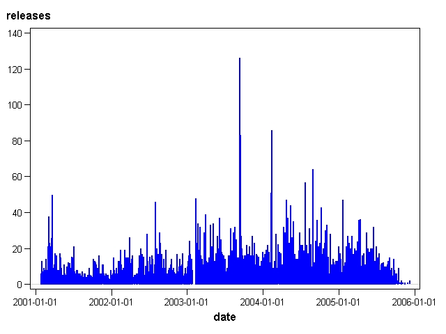
The following charts explore the effect of this censoring: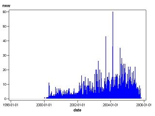

The first chart plots the number of movies having an earliest rating date on each day of the observation period. Only movies with a release year of 2000 or later are included so none of the data is censored. Although the chart is quite spiky, there is nothing special about the first few days, and the overall distribution is similar to the overall distribution of rating counts.

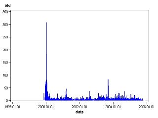
The second chart shows the distribution of earliest observed ratings for movies with release years prior to 2000. There are two interesting things to note. First, the large spike on the left represents movies that were already available for rating prior to the observation period. Second, although all these movies have release dates prior to 2000, the earliest rating dates are distributed across the five-year window similarly to the new releases. This suggests that old movies were becoming available on Netflix at a fairly steady rate across the observation period. At some time in the future, there will be no old movies left to release so all newly available movies will be new. Such shifts in the mixture over time can have a dramatic effect on predictions of future behavior.

Earliest ratings for new and old movies shown together on the same scale: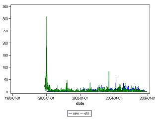

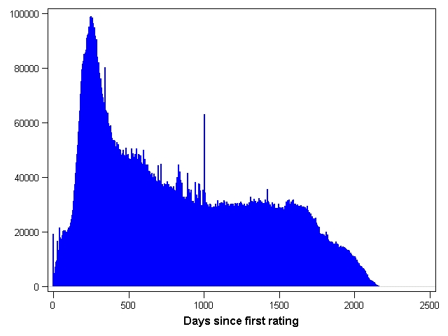
Intensity of rating activity by time since first rating

Originally posted to a previous version of this blog on 29 May 2007.

Many people in the Netflix sample rate movies one day and then never rate again. Overall, rating frequency declines over time. In this post, I look at what happens to the probability of making a rating as a function of tenure calculated as days elapsed since the subscriber's first rating. The first chart shows the raw count of ratings by tenure of the subscriber making the rating.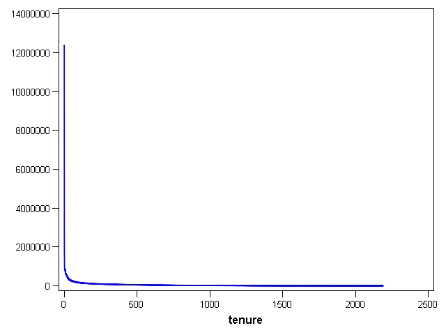



The query that produced this table is:



The reason for restricting the results to tenures shorter the 2,190 days is that beyond that ratings are so infrequent that some tenures are not even represented.

While this chart does show clearly that day 0 ratings are by far the most common (by definition, everyone in the training data made ratings on day 0), not much else is visible. In the second chart, the base 10 log of the ratings count is plotted. On this scale, we can see that after an initial percipitous decline, the number of ratings diminishes more slowly of the next 2,000 days and then drops off sharply as we run out of examples of subscribers with very high tenures.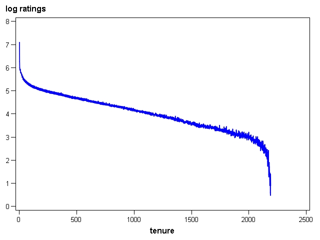



Recall that the earliest rating date in the training data is 11 November 1999 and the latest is 31 December 2005. This means that the theoretical highest observable tenure would be 2,242 days for a subscriber who submitted ratings on the first and last days of the observation period.

The raw count of ratings by tenure is not particularly informative on its own, but it is the first step towards calculating something quite useful: what is the expected number of ratings that a subscriber will make at any given tenure. This can be estimated empirically by dividing the actual count of ratings for each tenure by the number of people who ever experienced that tenure.This is reminiscent of estimating the hazard probability in survival analysis except that one can rate many movies on a single day and making a rating at tenure t is not conditional on not having made a rating at some earlier tenure. You only die once, but you can make ratings as often as you like. For this purpose, I assume that a subscriber comes into existence when he or she first rates a movie and remains eligible to make ratings for ever. In real life, of course, a subscriber could cease to be a Netflix customer, but that does not concern me as that is just one of several reasons that customers are less likely to make ratings over time. For the 2007 KDD Cup challenge, there is no requirement to predict whether customers cancel their subscriptions; only whether they keep rating movies.

The heart of the calculation combines the table created above with another table containing the number of subscribers who ever experienced each tenure.



On the first day that people rate movies, they rate a lot of them--over 25 on average. By the next day, their enthusiasm has waned dramatically.



The chart shows the expected number of ratings per day after the first 10 days.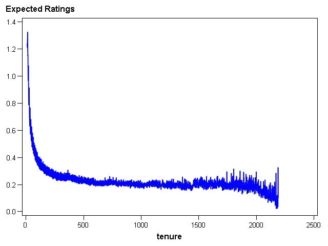



It is not surprising that the variance of the expected number of ratings gets high for higher tenures. The pool of people who have experienced the higher tenures is quite small as seen below.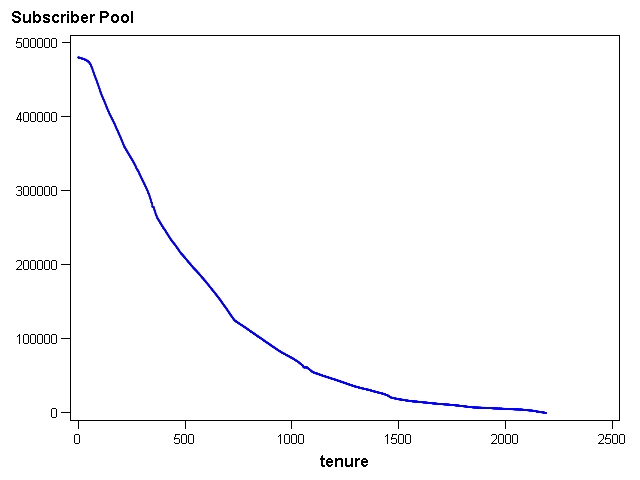

Netflix rating activity over time

This post was salvaged from the wreckage of a former version of the Data Miners blog. It was part of a series of postings on the data used for the Netflix competition. The original posting date was 12 May 2007. At that time, the 2007 KDD Cup competition was active. One of the tasks was to predict how many ratings would be made in 2006 by a group of raters observed through 2005 rating a group of movies that were all released during or before the observation period. Although the KDD contest has come and gone, the subject of how rating activity changes over time remains interesting.

In this post, I begin to look at what happens to a movie's propensity to be rated as a function of time since first availability. To avoid having to deal with the issue of interval censoring that I brought up in a previous post, I restrict my attention to movies that were first rated after 01 February 2000, well into the observation period. This first chart shows the raw, unadjusted count of ratings for all movies first rated after 01 February 2000 by days since first rating.

Raw count of ratings by movie age (days since first rating)

It is tempting to dive right in and start trying to interpret this raw data (what in the world is going on at day 1003? for example), but that temptation might lead to erroneous conclusions. There are two important things to keep in mind:

1. The number of raters is not constant over time. As the customer base grows, we can expect more rating activity so the absolute number of ratings a movie receives over time may not decay as quickly as it would for a fixed population. During the observation period, the number of raters grew substantially. For the KDD Cup task, on the other hand, we will be looking at the activity of a shrinking subpopulation. (Some customers who were active in the observation period are bound to quit, die, move away, or loose interest in making ratings; their replacements do not show up in our data.)


2. As the days since first rating number gets higher and higher, our data on rating behavior is based on a smaller and smaller number of movies. By definition, all the many thousands of movies in our sample experienced day 0. All but the few first rated on the last day of the observation period also experienced day 1. By the time we get to day 2000, only a handful of movies released in February of 2000 remain in the sample. Small numbers mean high variance. Also, as the time since first rating gets longer, the actual dates of first rating come from a narrower and narrower window, exposing us to seasonal effects that are averaged away for "younger" movies.

Change in rating activity over the observation period

In the next chart, I have adjusted the raw number of ratings received for each day since a movie was first rated to take into account the overall level of rating activity on that day. Since the Nth day since first rating comes on a different calendar date for each movie, this adjustment is made at the level of the rating transaction table before summarization. The adjustment is to count each rating as 1 over the total number of ratings that day.

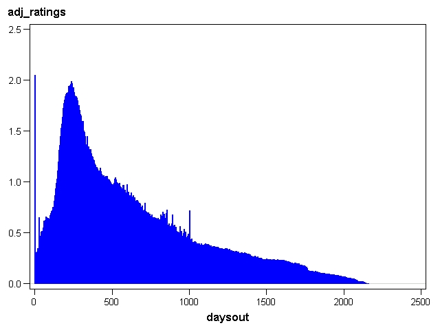Rating intensity over time adjusted for number of raters

The query to produce the data for both the unadjusted and adjusted charts is shown here:

One interesting feature is the high number of ratings on the first day of availability for rating. I suspect this represents people who see movies in theaters and are impatient to rate them when they are first available on Netflix. After that initial burst, I suspect that rating volume is largely a function of the number of disks in circulation for a newly released DVD. This appears to ramp up quickly. After a peak at around 230 days, a movie's rating activity goes into decline.

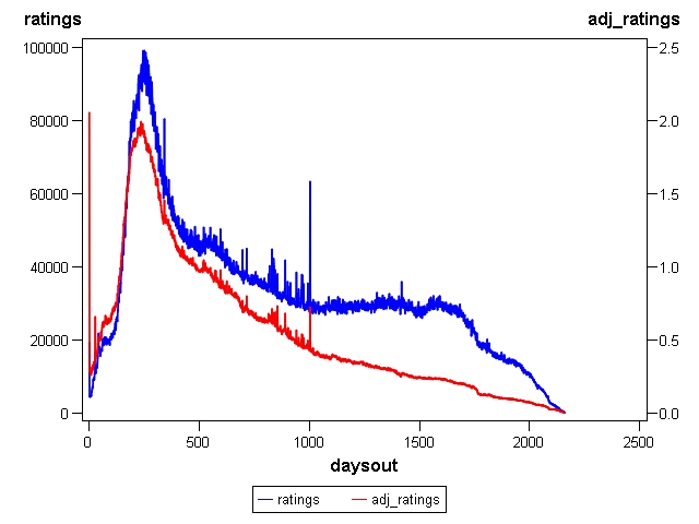Comparison of adjusted and unadjusted rating intensity

What of the effect of the declining number of movies for large values of days since first rating? The following chart shows the number of movies with earliest rating dates after 01 February 2000 that experienced each number of days since first rating.

As can be seen on the chart below, movies became available for rating throughout the period of 02 February 2005 through the end of 2005.

Movies newly available for rating by date

*How many movies of each age were available to be rated?
data atrisk(keep=daysout available);
set releases;
retain available decrease;
daysout = _N_-1;
if daysout = 0 then available=15405;
else available= available-decrease;
decrease=releases;
run;

*Rating activity by days available adjusted for size of pool
proc sql;
create table ratetenure_adj as
select l.daysout, l.ratings,
     l.ratings/r.available as rpm,
     l.adj_ratings/r.available as arpm
from ratetenure3 l, atrisk r
where l.daysout = r.daysout and r.available > 100
order by l.daysout;

The code above is in SAS. For the most part, I restrict myself to PROC SQL which is close enough to regular SQL that I do not bother to provide any explanation. This data step code is admittedly a bit odd, however. Had I followed my usual practice of storing my data in J arrays, things like subtracting a cumulative sum from an initial constant would be trivially accomplished using a scan expression such as c-+/\releases.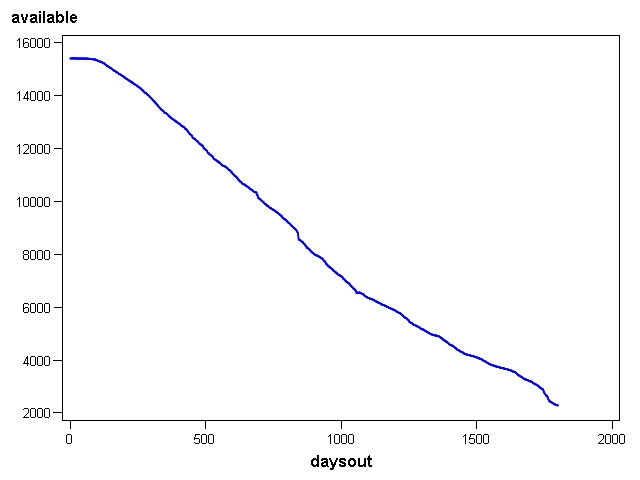

At the moment, however, the data is sitting in SAS tables. Given a table RELEASES containing the number of movies that became available on each date in reverse chronological order, I want to know how many movies were available for rating at each "age" where age is defined as days since the movie was first rated. A total of 15,402 movies became available for rating in the period from 02 February 2000 and the end of 2005. Any one of these movies could have been rated on its day 0 (which I am calling the "release date" although in fact, it is just the earliest rating date which might or might not be the same thing). The last day that any movies were released was 09 December 2005. I therefore consider that the end of the ratings window. The two movies released that day were not available to be rated at age 1 day because they did not achieve age 1 day within the window. All the rest of the movies were available to be rated at age 1. All movies released before the last two days of the window were available to be rated on both day 0 and day 1, and so forth.

Number of movies available for rating by age

In the chart below, the blue line shows absolute ratings per movie by movie "age." The red line shows ratings per movie by movie age adjusted for the overall growth in rating activity.

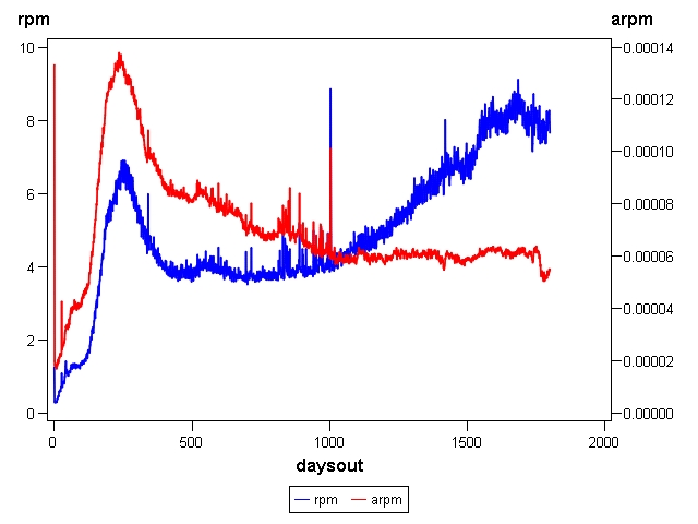Rating intensity by age of movie

A plea for comments
I find it quite surprising that the large spike in number of ratings that is visible on the calendar time line seems to survive translation to the days since first rating time line. My initial hypothesis about spikes on the calendar time line is that they represent glitches in the system where, for example, several days worth of rating activity got posted all at once. That sort of thing would disappear when moved to the days since first rating time line since the movies rated on a particular date are all at different ages. A spike on the days since first rating time line suggests that all the extra rating activity was around a single movie (that happens to had been available for rating for 1003 days when the event occurred) or that something else is going on that I haven't thought of. If anyone out there knows what is going on, please post a comment.