Writing to a text file from SQL Server

It has been a while since I've contributed to the blog . . . not because I've had nothing to say. In this time, I've been spending a lot of time working with SQL Server, producing useful stored procedures (and insights). In this post, I discuss one of them, a stored procedure in SQL Server to write text to a file.

This stored procedure is a utility. I learned a lot along the way while trying to write it. This post is intended to explain these learnings.

The approach that I'm taking is to use xp_cmdshell to write one line at a time using the DOS echo command. A different approach uses OLE automation and the File System Object. I couldn't get this to work, possibly because it requires configurations that I don't know about; possibly because I don't have the right permissions.

My stored procedure is called usp__AppendToFile and the code is at the end of this post. If you care about naming conventions, here is the reasoning behind the name. The "usp" prefix is for user stored procedure. Starting a stored procedure with usp or sp seems redundant to me, but appears to be a common and perhaps even a best practice. The double underscore is my convention, saying that this is a utility. It is then followed by a reasonable name.

usp__AppendToFile does the following: It takes a string (varchar(max)) and an optional end-of-line character. It then writes the string, one line at a time, using the echo command in DOS. By passing in the end of line character, the stored procedure can work with text that uses the DOS standard end of line (carriage return followed by line feed, the default) as well as other standards.

Although seemingly simple and using familiar tools, I learned several things from this effort.

My first lesson is that in order to write to a file, you need to be able to access it. When running you a command in SQL Server, it is not really "you" that needs permissions. The SQL Server service needs to be able to access the file. And this depends on the user running the service. To see this user, go to the Control Panel, choose the Administrative Tools, and select Services. Scroll down to find the SQL Server service (called something like SQL Server Agent), and look in the column Log On As.

As an example, the user running the service on one machine used a local machine account rather than a Windows verified domain account. For this reason, SQL Server could not access files on the network. Changing the service to run on a Windows-authenticated enabled SQL Server to create a file. (The alternative of changing the permissions for the user was not possible, since I do not have network sys admin privileges.)

The second lesson is that in order to write to a file using xp_cmdshell, you need to have xp_cmdshell enabled as shown here. There are good reasons why some DBAs strongly oppose enabling this option, since it does open up a security hole. Well, actually, the security hole is the fault of Microsoft, since the command is either enabled or disabled at the server level. What we really want is to give some users access to it, which denying others.

Third, the DOS way to write text to a file is using the echo command. Nothing is as simple as it seems. Echo does generally write text. However, it cannot write an empty line. Go ahead. Open a CMD shell, type in echo and see what happens. Then type in echo with a bunch of spaces and see what happens. What you get is the informative message: ECHO is on. Thanks a bunch, but that's not echoing what was on the command line.

I want my procedure to write blank lines when it finds them in the string. To fix this problem, use the echo. command. For whatever reason, having the period allows an empty line to be written. Apparently, other characters work as well, but period seems to be the accepted one.

The problems with DOS seem solved, but they are not. DOS has another issue: some special characters are interpreted by DOS, even before echo gets to them. For instance, > is interpreted to put the results to a file; | is interpreted as a pipe between commands, and & is interpreted as a background command. Fortunately, these can be escaped using the DOS escape character, which I'm sure everyone knows is a caret (^).

But, this issue does not end there, because special characters might be in a string, in which case they do not need to be escaped. Parsing a string in a stored procedure to find quotes is beyond the range of this stored procedure. Instead, if there are no double quotes in the string, then it escapes special characters. Otherwise, it does not.

Combining these lessons, here is what I consider to be a useful utility to write a string to a text file, even when the string consists of multiple lines.

CREATE procedure usp__AppendToFile (
   @str varchar(max),
   @FileName varchar(255),
   @EOL varchar(10) = NULL
) as
begin
   if @EOL is NULL
   begin
       set @EOL = char(13) + char(10);
   end;

   -- the period allows for empty lines
   declare @prefix varchar(255) = 'echo.';
   declare @suffix varchar(255) = '>>'+@FileName;

   -- Escape special characters so things work
   -- But escapes work funny when in double quotes (and maybe single quotes too)
   set @str = (case when charindex('"', @str) = 0
                    then replace(replace(replace(@str, '|', '^|'), '>', '^>'), '&', '^&')
                    else @str
               end);

   while (@str <> '')
   begin
       declare @pos int = charindex(@EOL, @str);
       declare @line varchar(8000) = (case when @pos > 0 then left(@str, @pos) else @str end);
       set @str = (case when @pos > 0 then substring(@str, @pos+2, 1000000) else '' end);

       set @line = @prefix+@line+@suffix;

       --write @line to file;
       exec xp_cmdshell @line;

   end;
end;  -- usp__AppendToFile

The Average Hotel Does Not Get The Average Rating

The millions of travelers who review hotels, restaurants, and other attractions on TripAdvisor also supply a numeric rating by clicking one of five circles ranging from 1 for "terrible" to 5 for "excellent." On the whole, travelers are pretty kind.The average review rating for hotels and other lodgings is over 3.9. The median score is 4 and since that middle review is lost somewhere in a huge pile of 4-ratings, well over half of hotel reviews give a 4 or 5 rating.

So with such kind reviewers, most hotels must have a rating over 4 and hoteliers must all love us, right? Actually, no. The average of all hotel ratings is 3.6. Here's why: some large, frequently-reviewed hotels have thousands of reviews. It is hardly surprising that the Bellagio in Las Vegas has about 250 times more reviews than say, the Cambridge Gateway Inn, an unloved motel in Cambridge, Massachusetts. It may or may not be surprising that these oft-reviewed properties tend to be well-liked by our reviewers. Surprising or not, it's true: the hotels with the most reviews have a higher average rating than the long tail of hotels, motels, B&Bs, and Inns with only a handful of reviews each.

The chart compares the distribution of user review scores with the distribution of hotel average scores.

For the curious, here are the top 10 hotels on TripAdvisor by number of reviews:

Luxor Las Vegas

Majestic Colonial Punta Cana

Bellagio Las Vegas

MGM Grand Hotel and Casino

Excellence Punta Cana

Flamingo Hotel & Casino

Venetian Resort Hotel Casino

Hotel Pennsylvania New York

Excalibur Hotel & Casino

Treasure Island - TI Hotel & Casino

Not all of these are beloved by TripAdvisor users. The Hotel Pennsylvania drags the average down since it receives more ones than any other score. Despite that, as a group these hotels have a higher than average score. The moral of the story is that you can't extrapolate from one level of aggregation to another without knowing how much weight to give each unit. In the last US presidential election, the average state voted Republican, but the average voter voted Democrat.

Common Table Expressions

It's been a while since I posted. My new role at TripAdvisor has been keeping me pretty busy! My first post after a long absence is about a feature of SQL that I have recently fallen in love with. Usually, I leave it to Gordon to write about SQL since he is an expert in that field, but this particular feature is one that he doe not  write about in Data Analysis Using SQL and Excel. The feature is called common table expressions or, more simply, the WITH statement.

Common table expressions allow you to name a bunch of useful subquerries before using them in your main query. I think of the common table expressions as subquerries because that is what they usually replace in my code, but they are actually a lot more convenient than subquerries because they aren't "sub". They are there at the top level so your main query can refer to them as many times as you like anywhere in the query. In that way, they are more like temporary tables or views. Unlike tables and views, however, you don't have to be granted permission to create them, and you don't have to remember to clean them up when you are done. Common table expressions last only as long as the query is running.

An example will help show why common table expressions are so useful. Suppose (because it happens to be true) that I have a complicated query that returns a list of hotels along with various metrics. These could be as simple as the number of rooms, or the average daily rate, or the average rating by our reviewers, or it could be a complex expression to produce a model score. For this purpose, it doesn't matter what the metric is, what matters is that I want to compare "similar" properties for some definition of similar. The first few rows returned by my complicated query look something like this:



Similar hotels have the same value of feature and similar ranking. In fact, I want to compare each hotel with four others: The one with matching feature that is next above it in rank, the one with matching feature that is next below it in rank, the one with non-matching feature that is next above it in rank, and the one with non-matching feature that is next below it in rank. Of course, for any one hotel, some of these neighbors may not exist. The top ranked hotel has no neighbors above it, for instance.

My final query involves joining the result pictured above with itself four times using non-equi joins, but for simplicity, I'll leave out the matching and non-matching features bit and simply compare each hotel to the one above and below it in rank. The ranking column is dense, so I can use equi joins on ranking=ranking+1 and ranking=ranking-1 to achieve this. Here is the query:

with ranks (id, hotel, ranking, feature, metric1, metric2)
    as(select . . .) /* complicated query to get rankings */
select r0.id, r0.hotel, 
    r0.metric1 as m1_self, r1.metric1 as m1_up, r2.metric1 as m1_down
from ranks r0 /* each hotel */ left join
      ranks r1 on r0.ranking=r1.ranking+1 /* the one above */ left join
      ranks r2 on r0.ranking=r2.ranking-1 /* the one below */
order by r0.ranking

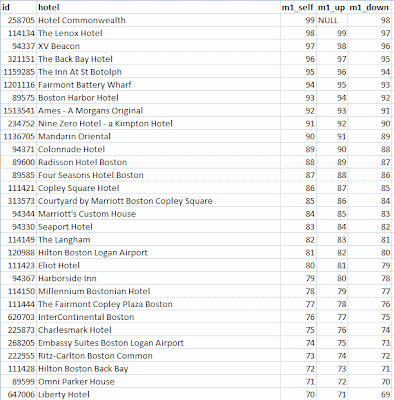
The common table expression gives my complicated query the name ranks. In the main query, ranks appears three times with aliases r0, r1, and r2. The outer joins ensure that I don't lose a hotel just because it is missing a neighbor above or below. The query result looks like this:

The Hotel Commonwealth has the highest score, a 99, so there is nothing above it. In this somewhat contrived example, the hotel below it is the Lenox with a score of 98 and so on down the list. To write this query using subqueries, I would have had to repeat the subquery three times which would not only be ugly, it would risk actually running the subquery three times since the query analyzer might not notice that they are identical.

JMP Webcast:: Measuring What Matters

On Tuesday, May 24 at 1:00pm Eastern Daylight Time, I will be presenting a webcast on behalf of JMP, a visual data exploration and mining tool.  The main theme of  the talk is that companies tend to manage to metrics, so it is very important that the metrics are well-chosen. I will illustrate this with a small case study from the world on on-line retailing recommendations. A secondary theme is the importance of careful data exploration in preparation for modeling--a task JMP is well-suited to.

-Michael

Register.

Michael Berry announces a new position

Hello Readers,

As some of you will already have heard, I have accepted the position of Business Intelligence Director at TripAdvisor for Business--the part of TripAdvsor that sells products and services to businesses rather than consumers. The largest part of T4B as this side of the business is called internally is selling direct links to hotel web sites that appear right next to the hotel reviews on TripAdvisor.com. Subscribers are also able to make special offers ("free parking", "20% off", "a free bottle of wine with your meal", . . .) directly on the TripAdvisor site. Another T4B product is listings for vacation rental properties.  There is a lot of data, and a lot of questions to be answered!

I will continue to contribute to this blog and I will continue to work with Gordon and Brij on the data mining courses that Data Miners produces. TripAdvisor is based in Newton, Massachusetts--not far from my home in Cambridge. It will be novel going home every night after work!

-Michael

Data Mining Techniques 3rd Edition

Gordon and I spent much of the last year writing the third edition of Data Mining Techniques and now, at last, I am holding the finished product in my hand. In the 14 years since the first edition came out, our knowledge has increased by a factor of at least 10 while the page count has only doubled so I estimate the information density has increased by a factor of five! I hope reviewers will agree that our writing skills have also improved with time and practice. In short, I'm very proud of our latest effort and I hope our readers will continue to find it useful for the next 14 years!

Table of Contents
Chapter 1 What Is Data Mining and Why Do It? 1
Chapter 2 Data Mining Applications in Marketing and Customer Relationship Management 27
Chapter 3 The Data Mining Process 67
Chapter 4 Statistics 101: What You Should Know About Data 101
Chapter 5 Descriptions and Prediction: Profi ling and Predictive Modeling 151
Chapter 6 Data Mining Using Classic Statistical Techniques 195
Chapter 7 Decision Trees 237
Chapter 8 Artifi cial Neural Networks 283
Chapter 9 Nearest Neighbor Approaches: Memory-Based Reasoning and Collaborative Filtering 323
Chapter 10 Knowing When to Worry: Using Survival Analysis to Understand Customers 359
Chapter 11 Genetic Algorithms and Swarm Intelligence 399
Chapter 12 Tell Me Something New: Pattern Discovery and Data Mining 431
Chapter 13 Finding Islands of Similarity: Automatic Cluster Detection 461
Chapter 14 Alternative Approaches to Cluster Detection 501
Chapter 15 Market Basket Analysis and Association Rules 537
Chapter 16 Link Analysis 583
Chapter 17 Data Warehousing, OLAP, Analytic Sandboxes, and Data Mining 615
Chapter 18 Building Customer Signatures 657
Chapter 19 Derived Variables: Making the Data Mean More 695
Chapter 20 Too Much of a Good Thing? Techniques for Reducing the Number of Variables 737
Chapter 21 Listen Carefully to What Your Customers Say: Text Mining 777
Index 823

How to calculate R-squared for a decision tree model

A client recently wrote to us saying that she liked decision tree models, but for a model to be used at her bank, the risk compliance group required an R-squared value for the model and her decision tree software doesn't supply one. How should she fill in the blank? There is more than one possible answer.

Start with the definition of R-squared for regular (ordinary least squares) regression. There are three common ways of describing it. For OLS they all describe the same calculation, but they suggest different ways of extending the definition to other models. The calculation is 1 minus the ratio of the sum of the squared residuals to the sum of the squared differences of the actual values from their average value.

The denominator of this ratio is the variance and the numerator is the variance of the residuals. So one way of describing R-squared is as the proportion of variance explained by the model.

A second way of describing the same ratio is that it shows how much better the model is than the null model which consists of not using any information from the explanatory variables and just predicting the average. (If you are always going to guess the same value, the average is the value that minimizes the squared error.)

Yet a third way of thinking about R-squared is that it is the square of the correlation r between the predicted and actual values. (That, of course, is why it is called R-squared.)

Back to the question about decision trees: When the target variable is continuous (a regression tree), there is no need to change the definition of R-squared. The predicted values are discrete, but everything still works.

When the target is a binary outcome, you have a choice. You can stick with the original formula. In that case, the predicted values are discrete with values between 0 and 1 (as many distinct estimates as the tree has leaves) and the actuals are either 0 or 1. The average of the actuals is the proportion of ones (i.e. the overall probability of being in class 1).  This method is called Efron's pseudo R-squared.

Alternatively, you can say that the job of the model is to classify things.  The null model would be to always predict the most common class. A good pseudo R-squared is how much better does your model do? In other words, the ratio of the proportion correctly classified by your model to the proportion of the most common class.

There are many other pseudo R-squares described on a page put up by the statistical consulting services group at UCLA.