Lines and Circles and Logistic Regression

Euclidean geometry, formalized in Euclid's Elements about 2,300 years ago, is in many ways a study of lines and circles.  One might think that after more than two millennia, we have moved beyond such basic shapes particularly in a realm such as data mining.  I don't think that is so true.

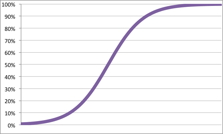
One of the overlooked aspects of logistic regression is how it is fundamentally looking for a line (or a plane or a hyperplane in multiple dimensions).  When most people learn about logistic regression, they start with an understanding of the sinuous curve associated with it (you can check out the Wikipedia page, for instance).  Something like this in one dimension:

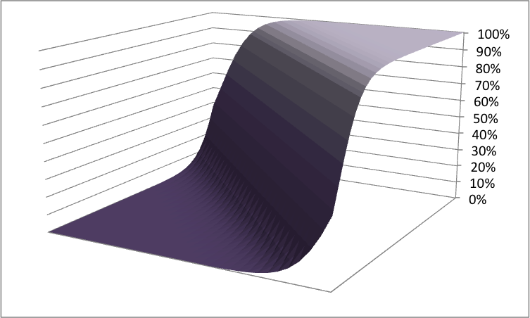
Or like this in two dimensions:

These types of pictures suggest that logistic regression is sinuous and curvaceous.  They are actually misleading.  Although the curve is sinuous and curvaceous, what is important is the boundary between the high values and the low values.  This separation boundary is typically a line or hyperplane; it is where the value of the logistic regression is 50%.  Or, assuming that the form of the regression is:

logit(x) = f(x) = a*x + y

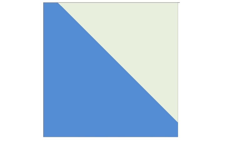
Then it is where the f(x) is set to 0.  What does this look like?   A logistic regression divides the space into two parts, one part to the "left" (or "above") the line/hyperplane and one part to the "right" (or "below").  A given line just splits the plane into two parts:

In this case, the light grey would be "0" (that is, less than 50%) and the blue "1" (that is, greater than 50%).  The boundary is where the logistic function takes on the value 50%.

Note that this is true even when you build a logistic regression sparse data.  For instance, if your original data has about 5% 1s and 95% 0s, the average value of the resulting model on the input data will be about 5%.  However, somewhere in the input space, the logistic regression will take on the value of 50%, even if there is no data there.  Even if the interpretation of a point in that area of the data space is non-sensical (the customer spends a million dollars a year and hasn't made a purchase in 270 years, or whatever).  The line does exist, separating the 0s from the 1s, even when all the data is on one side of that line.

What difference does this make?  Logistic regression models are often very powerful.  More advanced techniques, such as decision trees, neural networks, and support-vector machines, offer incremental improvement, and often not very much.  And often, that improvement can be baked back into a logistic regression model by a adding one or more derived variables.

What is happening is that the input variables (dimensions) for the logistic regression are chosen very carefully.  In a real situation (as opposed to the models one might build in a class), much thought and care has gone into the choice of variables and how they are combined to form derived variables.  As a result, the data has been stretched and folded in such a way that different classification values tend to be on different "side"s of the input space.

This manipulation of the inputs helps not only logistic regression but almost any technique.  Although the names are fancier and the computing power way more advanced, very powerful techniques rely on geometries studied 2,300 years ago in the ancient world.

Taking a Random Sample on Amazon Redshift

Recently, I was approached by Vicky whom I'm working with at a client, to help with a particular problem.  She wanted to calculate page view summaries for a random sample of visitors from a table containing about a billion page views.  This is a common problem, especially as data gets larger and larger.  Note that the sample itself is based on visitors, so a simple random sample is not sufficient.  We needed a sample of visitors and then all the pages for each visitor.

Along the way, I learned some interesting things about Redshift, taking random samples, and working with parallel and columnar databases.

For those not familiar with it, Redshift is an Amazon cloud data store that uses ParAccel, a parallel columnar database a based on Postgres (an older version of Postgres).  Postgres is a standard-enough relational databases, used by several database vendors as the basis of their products.

Columnar databases have interesting performance characteristics, because the database stores each column separately from other columns.  Although generally bad performance-wise for ACID-compliant transactions (if you don't know what ACID is, then you don't need to know), columnar databases are good for analysis.

However, your intuition about how things work may not apply.  A seemingly simple query such as this:

select *

from PageViews

limit 10;

takes a relatively long time (several minutes) because all the columns have to be read independently.  On the other hand, a query such as:

select min(BrowserId), max(BrowserId)
from PageViews;

Goes quite fast (a few seconds), because only one column has to be read into memory.  The more columns the queries reads, the slower it is -- other things being equal.

Back to the random sample.  A typical way of getting this type of random sample is to first find the reduced set of visitors and then join them back to the full page views.   This sounds cumbersome, but the strategy actually works well on many databases.  Applied to the query we were working with, the resulting query looks something like:

select pv.BrowserId,
from (select distinct BrowserId
      from PageViews
      order by random()
      limit 100000
     ) list join
     PageViews pv
     on list.BrowserId = pv.BrowserId
group by BrowserId;

This is a reasonable and standard approach to reduce the processing overhead.  The subquery list produces all the BrowserIds and then sorts them randomly (courtesy of the random() function).  The limit clause then takes a sample of one hundred thousand (out of many tens of millions).  The join would normally use an indexed key, so it should go pretty fast.  On Redshift, the subquery to get list performs relatively well.  But the entire query did not finish (our queries time out after 15-30 minutes). We experimented with a several variations, to no avail.

What finally worked?  Well, a much simpler query and this surprised us.  The following returned in just a few minutes:

select BrowserId,
from PageViews pv
group by BrowserId
order by random()
limit 100000;

In other words, doing the full aggregation on all the data and then doing the sorting is actually faster than trying to speed up the aggregation by working on a subset of the data.

I've been working with parallel databases for over twenty years.  I understand why this works better than trying to first reduce the size of the data.  Nevertheless, I am surprised.  My intuition about what works well in databases can be inverted when using parallel and columnar databases.

One of Vicky's requirements was for a repeatable random sample.  That means that we can get exactly the same sample when running the same query again.  The random() function does not provide the repeatability.  In theory, by setting the seed, it should.  In practice, this did not seem to work.  I suspect that aspects of load balancing in the parallel environment cause problems.

Fortunately, Postgres supports the md5() function.  This is a hash function that converts a perfectly readable string into a long string containing hexadecimal digits.  These digits have the property that two similar strings have produce very different results, so this is a good way to randomize strings.  It is not perfect, because two BrowserIds could have the same hash value, so they would always be included or excluded together.  But, we don't need perfection; we are not trying to land a little Curiousity lander in a small landing zone on a planet tens of millions of miles away.

The final form of the query was essentially:

select BrowserId,
from PageViews pv
group by BrowserId
order by md5('seed' || BrowserId)
limit 100000;

The constant "seed" allows us to get different, repeatable sample when necessary.  And Vicky can extract her sample in just a few minutes, whenever she wants to.

What will I do on my Caribbean vacation? Teach data mining, of course!

Monday, November 18th at the Radisson Hotel Barbados. Presented by Michael Berry of Tripadvisor and David Weisman of the University of Massachusetts.  Sponsored by Purple Leaf Communications. Registration and information here.

For Predictive Modeling, Big Data Is No Big Deal

That is what I will be speaking about when I give a keynote talk a the Predictive Analytics World conference on Monday, September 30th in Boston.

For one thing, data has always been big. Big is a relative concept and data has always been big relative to the computational power, storage capacity, and I/O bandwidth available to process it. I now spend less time worrying about data size than I did in 1980. For another, data size as measured in bytes may or may not matter depending on what you want to do with it. If your problem can be expressed as a completely data parallel algorithm, you can process any amount of data in constant time simply by adding more processors and disks.

This session looks at various ways that size can be measured such as number of nodes and edges in a social network graph, number of records, number of bytes, or number of distinct outcomes, and how the importance of size varies by task. I will pay particular attention to the importance or unimportance of data size to predictive analytics and conclude that for this application, data is powerfully predictive, whether big or relatively small. For predictive modeling, you soon reach a point where doubling the size of the training data has no effect on your favorite measure of model goodness. Once you pass that point, there is no reason to increase your sample size. In short, big data is no big deal.

Catch our Webcast on November 15

Gordon and I rarely find ourselves in the same city these days, but on November 15 we will be in Cary, North Carolina with our friends at JMP for a webcast with Anne Milley.  The format will be kind of like the first presidential debate with Anne as the moderator, and kind of like the second one with questions from you, the audience.  Sign up here.

Upcoming Speaking Engagements

After taking a break from speaking at conferences for a while, I will be speaking at two in the next month. Both events are here in Boston.

This Friday (9/14)  I will be at Big Data Innovation talking about how Tripadvisor for Business models subscriber happiness and what we can do to improve a subscriber's probability of renewal.

On October 1 and 2 I will be at Predictive Analytics World in Boston. This has become my favorite data mining conference. On the Monday, I will be visiting with my friends at JMP and giving a sponsored talk about how we use JMP for cannibalization analysis at Tripadvisor for Business. On Tuesday, I will go into the details of that analysis in more detail in a regular conference talk.

Measuring Site Engagement: Pages or Sessions

One of our clients is a large media website that faced a simple question: What is the best way to find the most engaged users on the web site? The goal was to focus a marketing effort on these users.

A media web site is challenging, because there is no simple definition of engagement or customer worth. The idea is that engagement can either lead to more advertising views or to longer subscriptions, depending on the business model for the site. On the other hand, for a retailing site, the question is simpler, because there is a simple method to see who the best customers are. Namely, the amount of money they spend.

Engagement is a nice marketing concept, but how can it be defined in the real world? One way is to simply look at the number of page views during some period of time. Another is to look at the number of sessions (or alternatively days of activity if sessions are not available) during a specified period of time. Yet another is to measure breadth of usage of the site over a period of time: Does the user only go to one page? Is the user only coming in on referrals from Google?

The first analysis used one month of data to define engagement. The top users for one month were determined based on pages and sessions. Of course, there is a lot of overlap between the two groups -- about 60% of the top deciles overlapped.

Which group seems better for defining engagement, the top users by page views or by sessions? To answer this, let's borrow an idea from survival and measure how many users are still around nine months later. (Nine months is arbitrary in this case). In this case, the return rate for the top decile for sessions was 74.4% but for the top decile for pages was lower at 73.8%. Not a big difference, but one that suggests that sessions are better.

Actually, the results are even more striking for visitors who are not in both top deciles. For the non-overlapping group, the session return rate is69.6% versus 67.9% for the page deciles.

For defining engagement, we then extended these results to three months instead of one to find the top one million most engaged users. The three measures are:

1. Visitors that have the most page views over three months.
2. Visitors that have the most sessions over three months.
3. Visitors in the top tercile of sessions (third) in each month, then take the highest terciles.

Three months was chosen as a rather arbitrary length of time, because the data was available. Holding it constant also lets us understand the difference between sessions and page views.

These three methods all produced about the same number of visitors -- the goal was to find the top one million most engaged users.

By these measures, the top one million visitors chosen by the three methods had the following "return" rates, nine months later:

1. Page views in three months: 65.4%
2. Sessions in three months: 65.9%
3. Sessions over three months: 66.9%

The nine-month survival suggests that the sessions over three months is the better approach for measuring engagement.